How can I help you?
Spreadsheet Data Presentation
Data presentation is helpful for proper representation of data in Spreadsheet. You have following features in Data Presentation.
- Cell types
- Chart
- Conditional formatting
- Filtering
- Pivot table
- Sorting
- Table
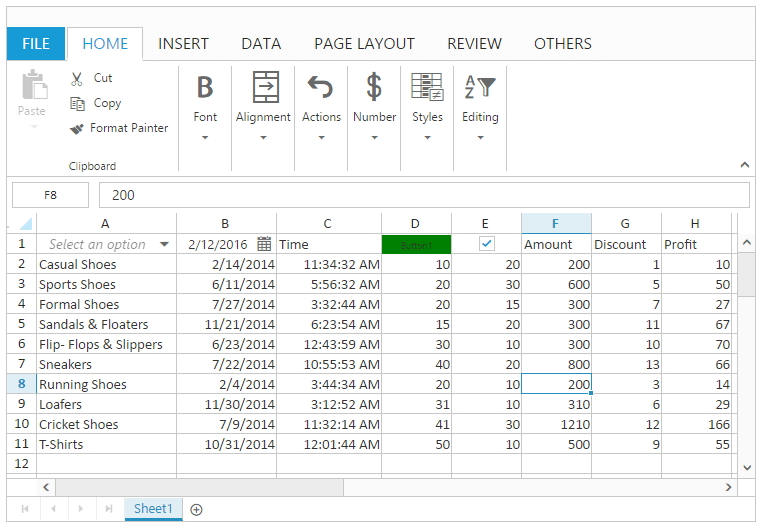
Cell Type
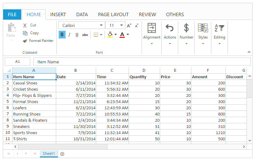
You can insert the controls like Button, Checkbox, Dropdown list and Date picker. You can use allow-cell-type property to enable/disable cell type operations.
To insert a Cell Type.
You can insert the cell type to the selected range of cells by one of the following ways
- Using
e-cell-typesproperty in sheets. - Using
addCellTypesmethod.
To remove Cell Type
You can delete the cell type in the selected range of cells by using removeCellTypes method.
The following code example describes the above behavior.
<ej-spread-sheet id="Spreadsheet" allow-cell-type="true" load-complete="loadComplete">
    <e-sheets>
        <e-sheet>
            <e-range-settings>
                <e-range-setting datasource ="ViewBag.Datasource"></e-range-setting>
            </e-range-settings>
            <e-cell-types>
                <e-cell-type range="A1">
                    <e-settings type="DropDownList" datasourcerange="A2:A11"></e-settings>
                </e-cell-type>
                <e-cell-type range="D1">
                    <e-settings type="Button" text="Button1" background-color="green"></e-settings>
                </e-cell-type>
                <e-cell-type range="C1">
                    <e-settings type="DropDownList" datasourcerange="A2:A11"></e-settings>
                </e-cell-type>
            </e-cell-types>
        </e-sheet>
    </e-sheets>
</ej-spread-sheet>

<script type="text/javascript">
    function loadComplete(args) {
        var xlCellType = this.XLCellType;
        if (!this.isImport) {
            xlCellType.addCellTypes("B1", {"type" : ej.Spreadsheet.CustomCellType.DatePicker, 'value' : '2/12/2016'},  1);
            xlCellType.addCellTypes("E1", {"type" : ej.Spreadsheet.CustomCellType.CheckBox, "isChecked" : true },  1);
            this.XLCellType.removeCellTypes("C1");
        }
    }
</script>
namespace samplebrowser.Controllers.SpreadsheetASP
{
public partial class SpreadsheetController : Controller
{
public ActionResult Default()
{
List<ItemDetail> lItems = new List<ItemDetail>();
lItems.Add(new ItemDetail() { ItemName = "Casual Shoes", Date = new DateTime(2014, 02, 14), Time = new DateTime(2014, 02, 14, 11, 34, 32), Quantity = 10, Price = 20, Amount = 200, Discount = 1, Profit = 10 });
lItems.Add(new ItemDetail() { ItemName = "Sports Shoes", Date = new DateTime(2014, 06, 11), Time = new DateTime(2014, 06, 11, 05, 56, 32), Quantity = 20, Price = 30, Amount = 600, Discount = 5, Profit = 50 });
lItems.Add(new ItemDetail() { ItemName = "Formal Shoes", Date = new DateTime(2014, 07, 27), Time = new DateTime(2014, 07, 27, 03, 32, 44), Quantity = 20, Price = 15, Amount = 300, Discount = 7, Profit = 27 });
lItems.Add(new ItemDetail() { ItemName = "Sandals & Floaters", Date = new DateTime(2014, 11, 21), Time = new DateTime(2014, 11, 21, 06, 23, 54), Quantity = 15, Price = 20, Amount = 300, Discount = 11, Profit = 67 });
lItems.Add(new ItemDetail() { ItemName = "Flip- Flops & Slippers", Date = new DateTime(2014, 06, 23), Time = new DateTime(2014, 06, 23, 12, 43, 59), Quantity = 30, Price = 10, Amount = 300, Discount = 10, Profit = 70 });
ViewBag.Datasource = lItems;
return View();
}
}
}The following output is displayed as a result of the above code example.
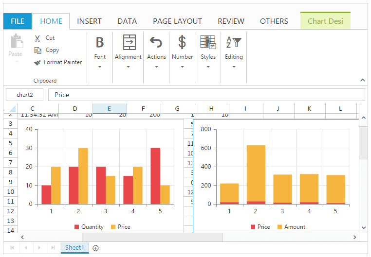
Chart
Chart is a graphical representation of data, that organizes and represents a set of numerical or qualitative data. It mostly displays the selected range of data in terms of x axis and y axis. You can use allow-charts property to enable/disable chart operations.
Types of Chart
The following types of charts are available in Spreadsheet.
- Area Chart
- Bar Chart
- Column Chart
- Line Chart
- Pie Chart
- Radar Chart
- Scatter Chart
You can create the Chart by one of the following ways,
- Using “Chart Type” button to Select the type of chart under Charts group of INSERT Tab in ribbon.
- Using
createChartmethod to create the chart.
Chart Customization
You can perform the following customizations for chart. These are available in DESIGN Tab which is enabled while clicking the chart element.
| Feature | Description |
|---|---|
| Add Chart Elements | You can add a chart element like chart axes, legends, chart title, axis title, data labels and grid lines. |
| Switch Row/Column | You can switch the row of the chart to column of the chart and vice versa. |
| Select Data | You can modify the data source of Chart. |
| Chart Type | You can change the type of the chart using Chart Type dialog. |
| Height and Width | You can change the height and width of the chart. |
| Chart Themes | You can change the theme of the chart. The available themes are saffron, lemon and azure in dark, light themes. |
The following code example describes the above behavior.
<ej-spread-sheet id="Spreadsheet" allow-charts="true"  load-complete="loadComplete">
    <e-sheets>
        <e-sheet>
            <e-range-settings>
                <e-range-setting datasource ="ViewBag.Datasource"></e-range-setting>
            </e-range-settings>
        </e-sheet>
    </e-sheets>
</ej-spread-sheet>

<script type="text/javascript">
    function loadComplete() {
        if (!this.isImport) {
            this.XLChart.createChart("D1:E6", { type: "column", enable3D: false, marker: false, top: 40, left: 260, width: 340, height: 250 });
            this.performSelection("E1");
            this.XLChart.createChart("E1:F6", { type: "stackingcolumn", enable3D: false, marker: { visible: false }, top: 40, left: 620, width: 340, height: 250 });
        }
    }
</script>
namespace samplebrowser.Controllers.SpreadsheetASP
{
public partial class SpreadsheetController : Controller
{
public ActionResult Default()
{
List<ItemDetail> lItems = new List<ItemDetail>();
lItems.Add(new ItemDetail() { ItemName = "Casual Shoes", Date = new DateTime(2014, 02, 14), Time = new DateTime(2014, 02, 14, 11, 34, 32), Quantity = 10, Price = 20, Amount = 200, Discount = 1, Profit = 10 });
lItems.Add(new ItemDetail() { ItemName = "Sports Shoes", Date = new DateTime(2014, 06, 11), Time = new DateTime(2014, 06, 11, 05, 56, 32), Quantity = 20, Price = 30, Amount = 600, Discount = 5, Profit = 50 });
lItems.Add(new ItemDetail() { ItemName = "Formal Shoes", Date = new DateTime(2014, 07, 27), Time = new DateTime(2014, 07, 27, 03, 32, 44), Quantity = 20, Price = 15, Amount = 300, Discount = 7, Profit = 27 });
lItems.Add(new ItemDetail() { ItemName = "Sandals & Floaters", Date = new DateTime(2014, 11, 21), Time = new DateTime(2014, 11, 21, 06, 23, 54), Quantity = 15, Price = 20, Amount = 300, Discount = 11, Profit = 67 });
lItems.Add(new ItemDetail() { ItemName = "Flip- Flops & Slippers", Date = new DateTime(2014, 06, 23), Time = new DateTime(2014, 06, 23, 12, 43, 59), Quantity = 30, Price = 10, Amount = 300, Discount = 10, Profit = 70 });
ViewBag.Datasource = lItems;
return View();
}
}
}The following output is displayed as a result of the above code example.
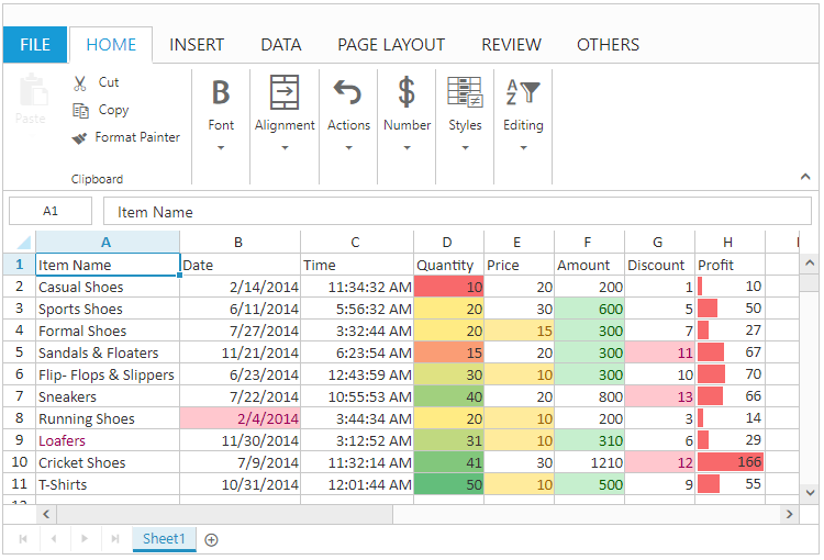
Conditional Formatting
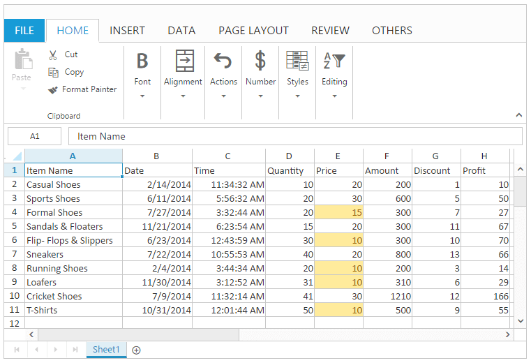
Conditional formatting helps you to apply formats to a cell or range with certain color based on the cells values. You can use allow-conditional-formats property to enable/disable Conditional formats.
Condition Definition
You can define conditions such as greater than, less than, between, equal to, text contains and date occurring for selected cells and defining value for condition. It highlights the specified cell.
You can do this by one of the following ways,
- Using “Conditional Formatting” option in Conditional Formatting button of HOME Tab in ribbon to open the conditional formatting dialog.
- Using
setCFRulemethod to define the condition.
The following code example describes the above behavior.
<ej-spread-sheet id="Spreadsheet" allow-conditional-formats="true"  load-complete="loadComplete">
    <e-sheets>
        <e-sheet>
            <e-range-settings>
                <e-range-setting datasource ="ViewBag.Datasource"></e-range-setting>
            </e-range-settings>
        </e-sheet>
    </e-sheets>
</ej-spread-sheet>

<script type="text/javascript">
    function loadComplete() {
        var xlCFormat = this.XLCFormat;
        if (!this.isImport) {
           xlCFormat.setCFRule({ "action": "greaterthan", "inputs": ["10"], "color": "redft", "range": "G2:G11" });
           xlCFormat.setCFRule({ "action": "lessthan", "inputs": ["20"], "color": "yellowft", "range": "E1:E11" });
           xlCFormat.setCFRule({ "action": "between", "inputs": ["300", "600"], "color": "greenft", "range": "F2:F11" });
           xlCFormat.setCFRule({ "action": "textcontains", "inputs": ["loafers"], "color": "redt", "range": "A1:A11" });
           xlCFormat.setCFRule({ "action": "dateoccur", "inputs": ["02/04/2014"], "color": "redft", "range": "B1:B11" });
		   xlCFormat.setCFRule({ "action": "databar", "color": "redft", "range": "H1:H11" });
           xlCFormat.setCFRule({action: "colorscale", color: "gyr", range: "D2:D11"});
        }
    }
</script>
namespace samplebrowser.Controllers.SpreadsheetASP
{
public partial class SpreadsheetController : Controller
{
public ActionResult Default()
{
List<ItemDetail> lItems = new List<ItemDetail>();
lItems.Add(new ItemDetail() { ItemName = "Casual Shoes", Date = new DateTime(2014, 02, 14), Time = new DateTime(2014, 02, 14, 11, 34, 32), Quantity = 10, Price = 20, Amount = 200, Discount = 1, Profit = 10 });
lItems.Add(new ItemDetail() { ItemName = "Sports Shoes", Date = new DateTime(2014, 06, 11), Time = new DateTime(2014, 06, 11, 05, 56, 32), Quantity = 20, Price = 30, Amount = 600, Discount = 5, Profit = 50 });
lItems.Add(new ItemDetail() { ItemName = "Formal Shoes", Date = new DateTime(2014, 07, 27), Time = new DateTime(2014, 07, 27, 03, 32, 44), Quantity = 20, Price = 15, Amount = 300, Discount = 7, Profit = 27 });
lItems.Add(new ItemDetail() { ItemName = "Sandals & Floaters", Date = new DateTime(2014, 11, 21), Time = new DateTime(2014, 11, 21, 06, 23, 54), Quantity = 15, Price = 20, Amount = 300, Discount = 11, Profit = 67 });
lItems.Add(new ItemDetail() { ItemName = "Flip- Flops & Slippers", Date = new DateTime(2014, 06, 23), Time = new DateTime(2014, 06, 23, 12, 43, 59), Quantity = 30, Price = 10, Amount = 300, Discount = 10, Profit = 70 });
ViewBag.Datasource = lItems;
return View();
}
}
}The following output is displayed as a result of the above code example.
Clear Rules
You can clear the defined rules by using one of the following ways,
- Using “Clear Rules” option in Conditional Formatting button of HOME Tab in ribbon to clear the rule.
- Using
clearCFmethod to clear the defined rules.
The following code example describes the above behavior.
<ej-spread-sheet id="Spreadsheet" allow-conditional-formats="true"  load-complete="loadComplete">
    <e-sheets>
        <e-sheet>
            <e-range-settings>
                <e-range-setting datasource ="ViewBag.Datasource"></e-range-setting>
            </e-range-settings>
        </e-sheet>
    </e-sheets>
</ej-spread-sheet>

<script type="text/javascript">
    function loadComplete() {
        var xlCFormat = this.XLCFormat;
        if (!this.isImport) {
            xlCFormat.setCFRule({ "action": "greaterthan", "inputs": ["10"], "color": "redft", "range": "G2:G11" });
            xlCFormat.setCFRule({ "action": "lessthan", "inputs": ["20"], "color": "yellowft", "range": "E1:E11" });
            xlCFormat.setCFRule({ "action": "between", "inputs": ["300", "600"], "color": "greenft", "range": "F2:F11" });
            xlCFormat.clearCF(true, "G2:G11");
            xlCFormat.clearCF(true, "F2:F11");
        }
    }
</script>
namespace samplebrowser.Controllers.SpreadsheetASP
{
public partial class SpreadsheetController : Controller
{
public ActionResult Default()
{
List<ItemDetail> lItems = new List<ItemDetail>();
lItems.Add(new ItemDetail() { ItemName = "Casual Shoes", Date = new DateTime(2014, 02, 14), Time = new DateTime(2014, 02, 14, 11, 34, 32), Quantity = 10, Price = 20, Amount = 200, Discount = 1, Profit = 10 });
lItems.Add(new ItemDetail() { ItemName = "Sports Shoes", Date = new DateTime(2014, 06, 11), Time = new DateTime(2014, 06, 11, 05, 56, 32), Quantity = 20, Price = 30, Amount = 600, Discount = 5, Profit = 50 });
lItems.Add(new ItemDetail() { ItemName = "Formal Shoes", Date = new DateTime(2014, 07, 27), Time = new DateTime(2014, 07, 27, 03, 32, 44), Quantity = 20, Price = 15, Amount = 300, Discount = 7, Profit = 27 });
lItems.Add(new ItemDetail() { ItemName = "Sandals & Floaters", Date = new DateTime(2014, 11, 21), Time = new DateTime(2014, 11, 21, 06, 23, 54), Quantity = 15, Price = 20, Amount = 300, Discount = 11, Profit = 67 });
lItems.Add(new ItemDetail() { ItemName = "Flip- Flops & Slippers", Date = new DateTime(2014, 06, 23), Time = new DateTime(2014, 06, 23, 12, 43, 59), Quantity = 30, Price = 10, Amount = 300, Discount = 10, Profit = 70 });
ViewBag.Datasource = lItems;
return View();
}
}
}The following output is displayed as a result of the above code example.
Filtering
Filtering allows you to view specific rows in Spreadsheet, while hiding the other rows. When a filter is added to the header row, a drop-down menu appears in each cell of the header row. You can use allow-filtering property to enable/disable filtering.
You can apply filtering by one of the following ways,
- Using “Filter” option in Sort & Filter button under Editing group of HOME Tab in ribbon.
- Using “Filter” button under Sort and Filter group of DATA Tab in ribbon.
You have following options in Filtering.
- Filter by Value.
- Filter by Color.
- Clear Filter.
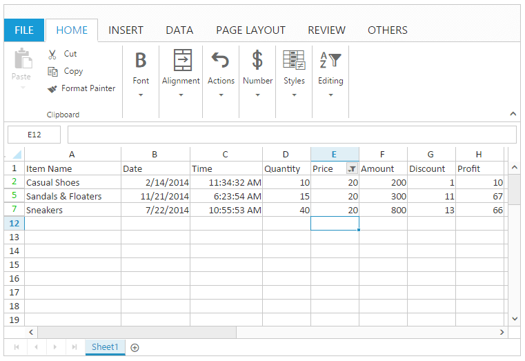
Filter by Value
You can perform filtering by using number, string. The filtered rows are only visible in the Spreadsheet. All the other rows within the filtered range were hidden.
You can do this by one of the following ways,
- Using dropdown button in filter header to open the filter dialog.
- Using context menu to select “Filter by Selected Cell’s Value” option in Filter.
- Using
filterByActiveCellmethod.
The following code example describes the above behavior.
<ej-spread-sheet id="Spreadsheet" allow-filtering="true"  load-complete="loadComplete">
    <e-sheets>
        <e-sheet>
            <e-range-settings>
                <e-range-setting datasource ="ViewBag.Datasource"></e-range-setting>
            </e-range-settings>
        </e-sheet>
    </e-sheets>
</ej-spread-sheet>

<script type="text/javascript">
    function loadComplete() {
        var xlFilter = this.XLFilter;
        if (!this.isImport) {
            this.performSelection("E2");
            xlFilter.filterByActiveCell();
        }
    }
</script>
namespace samplebrowser.Controllers.SpreadsheetASP
{
public partial class SpreadsheetController : Controller
{
public ActionResult Default()
{
List<ItemDetail> lItems = new List<ItemDetail>();
lItems.Add(new ItemDetail() { ItemName = "Casual Shoes", Date = new DateTime(2014, 02, 14), Time = new DateTime(2014, 02, 14, 11, 34, 32), Quantity = 10, Price = 20, Amount = 200, Discount = 1, Profit = 10 });
lItems.Add(new ItemDetail() { ItemName = "Sports Shoes", Date = new DateTime(2014, 06, 11), Time = new DateTime(2014, 06, 11, 05, 56, 32), Quantity = 20, Price = 30, Amount = 600, Discount = 5, Profit = 50 });
lItems.Add(new ItemDetail() { ItemName = "Formal Shoes", Date = new DateTime(2014, 07, 27), Time = new DateTime(2014, 07, 27, 03, 32, 44), Quantity = 20, Price = 15, Amount = 300, Discount = 7, Profit = 27 });
lItems.Add(new ItemDetail() { ItemName = "Sandals & Floaters", Date = new DateTime(2014, 11, 21), Time = new DateTime(2014, 11, 21, 06, 23, 54), Quantity = 15, Price = 20, Amount = 300, Discount = 11, Profit = 67 });
lItems.Add(new ItemDetail() { ItemName = "Flip- Flops & Slippers", Date = new DateTime(2014, 06, 23), Time = new DateTime(2014, 06, 23, 12, 43, 59), Quantity = 30, Price = 10, Amount = 300, Discount = 10, Profit = 70 });
ViewBag.Datasource = lItems;
return View();
}
}
}The following output is displayed as a result of the above code example.
Filter by Color
You can perform filtering by the selected cell color or font color. The filtered rows are only visible in the Spreadsheet. You can do this by clicking “Filter by Color” option in filter dialog to select filter by cell color or font color.
NOTE
This option is only available if the selected range of cells having any color.
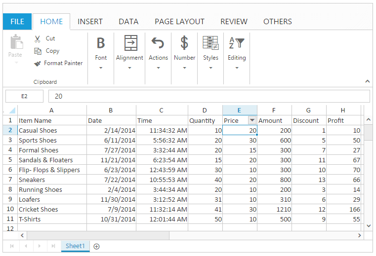
Clear Filter
You can clear the filtering to show all the filtered rows in the spreadsheet within the filtered range.
You can do this by one of the following ways,
- Using “Clear Filter” option in the filter dialog.
- Using context menu to select “Clear Filter” option in Filter.
- Using “Clear Filter” option in “Sort & Filter” button under Editing group of HOME Tab in ribbon.
- Using “Clear Filter” option under Sort and Filter group of DATA Tab in ribbon.
- Using
clearFiltermethod to perform clear filtering.
The following code example describes the above behavior.
<ej-spread-sheet id="Spreadsheet" allow-filtering="true"  load-complete="loadComplete">
    <e-sheets>
        <e-sheet>
            <e-range-settings>
                <e-range-setting datasource ="ViewBag.Datasource"></e-range-setting>
            </e-range-settings>
        </e-sheet>
    </e-sheets>
</ej-spread-sheet>

<script type="text/javascript">
    function loadComplete() {
        var xlFilter = this.XLFilter;
        if (!this.isImport) {
            this.performSelection("E2");
            xlFilter.filterByActiveCell();
            xlFilter.clearFilter();
        }
    }
</script>
namespace samplebrowser.Controllers.SpreadsheetASP
{
public partial class SpreadsheetController : Controller
{
public ActionResult Default()
{
List<ItemDetail> lItems = new List<ItemDetail>();
lItems.Add(new ItemDetail() { ItemName = "Casual Shoes", Date = new DateTime(2014, 02, 14), Time = new DateTime(2014, 02, 14, 11, 34, 32), Quantity = 10, Price = 20, Amount = 200, Discount = 1, Profit = 10 });
lItems.Add(new ItemDetail() { ItemName = "Sports Shoes", Date = new DateTime(2014, 06, 11), Time = new DateTime(2014, 06, 11, 05, 56, 32), Quantity = 20, Price = 30, Amount = 600, Discount = 5, Profit = 50 });
lItems.Add(new ItemDetail() { ItemName = "Formal Shoes", Date = new DateTime(2014, 07, 27), Time = new DateTime(2014, 07, 27, 03, 32, 44), Quantity = 20, Price = 15, Amount = 300, Discount = 7, Profit = 27 });
lItems.Add(new ItemDetail() { ItemName = "Sandals & Floaters", Date = new DateTime(2014, 11, 21), Time = new DateTime(2014, 11, 21, 06, 23, 54), Quantity = 15, Price = 20, Amount = 300, Discount = 11, Profit = 67 });
lItems.Add(new ItemDetail() { ItemName = "Flip- Flops & Slippers", Date = new DateTime(2014, 06, 23), Time = new DateTime(2014, 06, 23, 12, 43, 59), Quantity = 30, Price = 10, Amount = 300, Discount = 10, Profit = 70 });
ViewBag.Datasource = lItems;
return View();
}
}
}The following output is displayed as a result of the above code example.
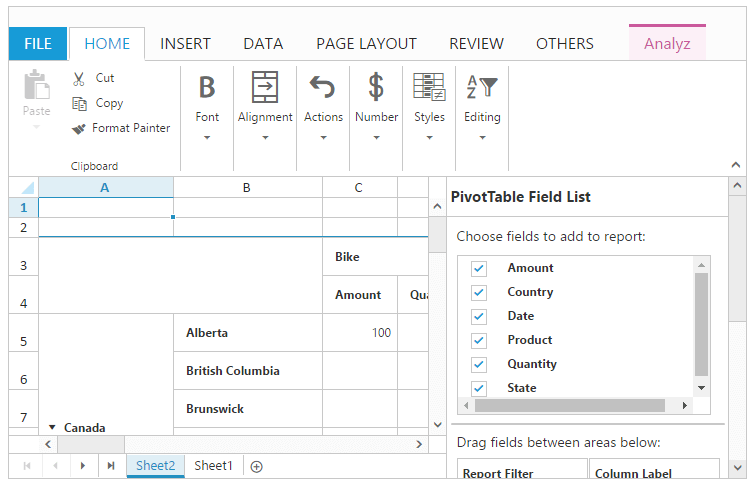
Pivot Table
Pivot table is a program tool that allows you to reorganize and summarize selected columns and rows of data to obtain a desired report. You can use enable-pivot-table property to enable/disable pivot table operations.
You can do this by one of the following ways,
- Using “Pivot Table” option under Tables group of INSERT Tab in ribbon.
- Using
createPivotTablemethod to create pivot table - Using
deletePivotTablemethod to remove the pivot table.
The following code example describes the above behavior.
<ej-spread-sheet id="Spreadsheet" enable-pivot-table="true"  load-complete="loadComplete">
    <e-sheets>
        <e-sheet>
            <e-range-settings>
                <e-range-setting datasource ="ViewBag.Datasource"></e-range-setting>
            </e-range-settings>
        </e-sheet>
    </e-sheets>
</ej-spread-sheet>

<script type="text/javascript">
    function loadComplete() {
        if (!this.isImport) {
            var settings = {
                rows: [{ fieldName: "Country" }, { fieldName: "State" }],
                columns: [{ fieldName: "Product" }],
                values: [{ fieldName: "Amount" }, { fieldName: "Quantity" }],
                filters: [{ fieldName: "Date" }]
            };
            this.XLPivot.createPivotTable("Sheet1!$A$1:$F$25", null, null, settings);
            //this.XLPivot.deletePivotTable("name");
        }
    }
</script>
namespace samplebrowser.Controllers.SpreadsheetASP
{
public partial class SpreadsheetController : Controller
{
public ActionResult Default()
{
List<PivotData> data = new List<PivotData>();
data.Add(new PivotData() { Amount = 100, Country = "Canada", Date = "FY 2005", Product = "Bike", Quantity = 2, State = "Alberta" });
data.Add(new PivotData() { Amount = 200, Country = "Canada", Date = "FY 2006", Product = "Van", Quantity = 3, State = "British Columbia" });
data.Add(new PivotData() { Amount = 300, Country = "Canada", Date = "FY 2007", Product = "Car", Quantity = 4, State = "Brunswick" });
data.Add(new PivotData() { Amount = 150, Country = "Canada", Date = "FY 2008", Product = "Bike", Quantity = 3, State = "Manitoba" });
data.Add(new PivotData() { Amount = 200, Country = "Canada", Date = "FY 2006", Product = "Car", Quantity = 4, State = "Ontario" });
data.Add(new PivotData() { Amount = 100, Country = "Canada", Date = "FY 2007", Product = "Van", Quantity = 1, State = "Quebec" });
data.Add(new PivotData() { Amount = 200, Country = "France", Date = "FY 2005", Product = "Bike", Quantity = 2, State = "Charente-Maritime" });
data.Add(new PivotData() { Amount = 250, Country = "France", Date = "FY 2006", Product = "Van", Quantity = 4, State = "Essonne" });
data.Add(new PivotData() { Amount = 300, Country = "France", Date = "FY 2007", Product = "Car", Quantity = 3, State = "Garonne (Haute)" });
data.Add(new PivotData() { Amount = 150, Country = "France", Date = "FY 2008", Product = "Van", Quantity = 2, State = "Gers" });
data.Add(new PivotData() { Amount = 200, Country = "Germany", Date = "FY 2006", Product = "Van", Quantity = 3, State = "Bayern" });
data.Add(new PivotData() { Amount = 250, Country = "Germany", Date = "FY 2007", Product = "Car", Quantity = 3, State = "Brandenburg" });
data.Add(new PivotData() { Amount = 150, Country = "Germany", Date = "FY 2008", Product = "Car", Quantity = 4, State = "Hamburg" });
data.Add(new PivotData() { Amount = 200, Country = "Germany", Date = "FY 2008", Product = "Bike", Quantity = 4, State = "Hessen" });
data.Add(new PivotData() { Amount = 150, Country = "Germany", Date = "FY 2007", Product = "Van", Quantity = 3, State = "Nordrhein-Westfalen" });
data.Add(new PivotData() { Amount = 100, Country = "Germany", Date = "FY 2005", Product = "Bike", Quantity = 2, State = "Saarland" });
data.Add(new PivotData() { Amount = 150, Country = "United Kingdom", Date = "FY 2008", Product = "Bike", Quantity = 5, State = "England" });
data.Add(new PivotData() { Amount = 250, Country = "United States", Date = "FY 2007", Product = "Car", Quantity = 4, State = "Alabama" });
data.Add(new PivotData() { Amount = 200, Country = "United States", Date = "FY 2005", Product = "Van", Quantity = 4, State = "California" });
data.Add(new PivotData() { Amount = 100, Country = "United States", Date = "FY 2006", Product = "Bike", Quantity = 2, State = "Colorado" });
data.Add(new PivotData() { Amount = 150, Country = "United States", Date = "FY 2008", Product = "Car", Quantity = 3, State = "New Mexico" });
data.Add(new PivotData() { Amount = 200, Country = "United States", Date = "FY 2005", Product = "Bike", Quantity = 4, State = "New York" });
data.Add(new PivotData() { Amount = 250, Country = "United States", Date = "FY 2008", Product = "Car", Quantity = 3, State = "North Carolina" });
data.Add(new PivotData() { Amount = 300, Country = "United States", Date = "FY 2007", Product = "Van", Quantity = 4, State = "South Carolina" });
ViewBag.Datasource = data;
return View();
}
}
}The following output is displayed as a result of the above code example.
Sorting
Sorting helps you to arrange the data to particular order in a selected range of cells. You can use allow-sorting property to enable/disable sorting.
You have following options in sorting.
- Sort by Ascending or Descending.
- Sort by Color.
Sort by Ascending and Descending
You can perform number sorting by ascending or descending and string sorting by A to Z or Z to A to arrange the data.
You can do this by one of the following ways,
- By choosing “Sort A to Z” or “Sort Z to A” in Sort & Filter button under Editing group of HOME Tab in ribbon.
- Using “Sort A to Z” or “Sort Z to A” button in Sort & Filter group of DATA Tab in ribbon.
- Using context menu to select “Sort A to Z” or “Sort Z to A” for strings and option in Sort.
- Using “Sort A to Z” or “Sort Z to A” for strings an “Sort Smallest to Largest” or “Sort Largest to Smallest” for numbers in filter dialog.
- Using
sortByRangemethod.
The following code example describes the above behavior.
<ej-spread-sheet id="Spreadsheet" allow-sorting="true"  load-complete="loadComplete">
    <e-sheets>
        <e-sheet>
            <e-range-settings>
                <e-range-setting datasource ="ViewBag.Datasource"></e-range-setting>
            </e-range-settings>
        </e-sheet>
    </e-sheets>
</ej-spread-sheet>

<script type="text/javascript">
    function loadComplete() {
        var xlSort = this.XLSort, xlFormat = this.XLFormat;
        if (!this.isImport) {
            xlSort.sortByRange("A2:A10", "A", "ascending");
            xlSort.sortByRange("E2:E10", "E", "descending");
        }
    }
</script>
namespace samplebrowser.Controllers.SpreadsheetASP
{
public partial class SpreadsheetController : Controller
{
public ActionResult Default()
{
List<ItemDetail> lItems = new List<ItemDetail>();
lItems.Add(new ItemDetail() { ItemName = "Casual Shoes", Date = new DateTime(2014, 02, 14), Time = new DateTime(2014, 02, 14, 11, 34, 32), Quantity = 10, Price = 20, Amount = 200, Discount = 1, Profit = 10 });
lItems.Add(new ItemDetail() { ItemName = "Sports Shoes", Date = new DateTime(2014, 06, 11), Time = new DateTime(2014, 06, 11, 05, 56, 32), Quantity = 20, Price = 30, Amount = 600, Discount = 5, Profit = 50 });
lItems.Add(new ItemDetail() { ItemName = "Formal Shoes", Date = new DateTime(2014, 07, 27), Time = new DateTime(2014, 07, 27, 03, 32, 44), Quantity = 20, Price = 15, Amount = 300, Discount = 7, Profit = 27 });
lItems.Add(new ItemDetail() { ItemName = "Sandals & Floaters", Date = new DateTime(2014, 11, 21), Time = new DateTime(2014, 11, 21, 06, 23, 54), Quantity = 15, Price = 20, Amount = 300, Discount = 11, Profit = 67 });
lItems.Add(new ItemDetail() { ItemName = "Flip- Flops & Slippers", Date = new DateTime(2014, 06, 23), Time = new DateTime(2014, 06, 23, 12, 43, 59), Quantity = 30, Price = 10, Amount = 300, Discount = 10, Profit = 70 });
ViewBag.Datasource = lItems;
return View();
}
}
}The following output is displayed as a result of the above code example.
Sort by Color
You can perform sort by color to arrange the data based on the selected cell’s background color or font color. This option is only available if the selected range of cells having any color.
You can do this by one of the following ways,
- Using “Sort By Color” option in filter dialog to perform sorting by cell color or font color.
- Using context menu to select “Put Selected Cell Color To The Top” or “Put Selected Font Color To The Top” in Sort option.
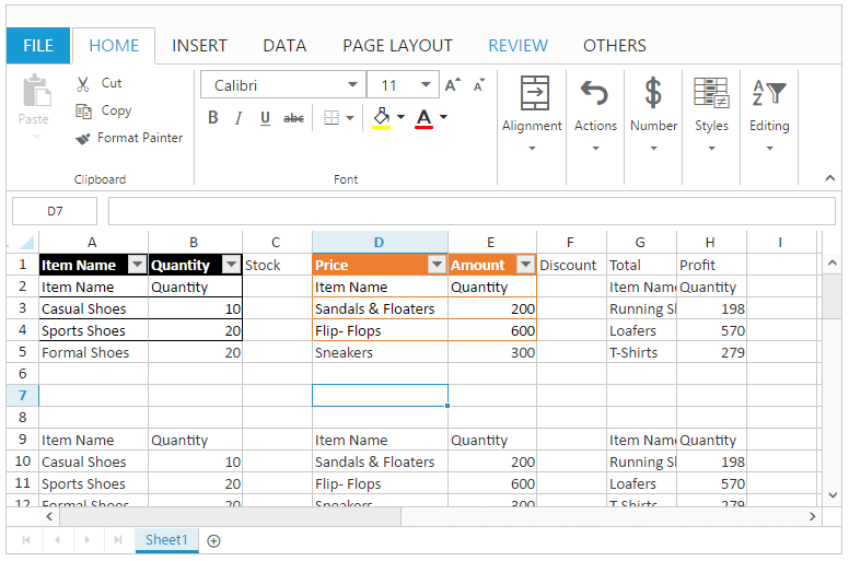
Table
A table is a data structure that organizes information into rows and columns. You can use allow-format-as-table property to enable/disable table operations.
You can do this by one of the following ways,
- Using “Format As Table” under Styles group of HOME Tab in ribbon.
- Using Table option under Tables group of INSERT Tab in ribbon.
- Using
createTablemethod to insert a table andremoveTableto delete a table.
Table Customization
You can perform the following customizations for table. These are available in DESIGN Tab which is enabled while clicking the table.
| Feature | Description |
|---|---|
| Resize Table | You can resize the table only to increase row count. |
| Convert to Range | You can remove the table using this option. |
| First Column | You can highlight the first column of the table. |
| Last Column | You can highlight the last column of the table. |
| Total Row | You can insert a new row in the bottom of the table to display the total value of the last column. You can toggle this by using checkbox. |
| Filter Button | You can able to hide or unhide the filter icons in the filter header of a table. |
The following code example describes the above behavior.
<ej-spread-sheet id="Spreadsheet" allow-format-as-table="true"  load-complete="loadComplete">
    <e-sheets>
        <e-sheet>
            <e-range-settings>
                <e-range-setting datasource ="ViewBag.Datasource"></e-range-setting>
            </e-range-settings>
        </e-sheet>
    </e-sheets>
</ej-spread-sheet>

<script type="text/javascript">
    function loadComplete(args) {
        var xlFormat = this.XLFormat;
        if (!this.isImport) {
            xlFormat.createTable({ "header": true, "formatName": "TableStyleLight8" }, "A1:B4");
            xlFormat.createTable({ "header": true, "formatName": "TableStyleLight10" }, "D1:E4");
        }
    }
</script>
namespace samplebrowser.Controllers.SpreadsheetASP
{
public partial class SpreadsheetController : Controller
{
public ActionResult Default()
{
List<FormatData> formats = new List<FormatData>();
formats.Add(new FormatData() { format1 = "Item Name", format2 = "Quantity", format4 = "Item Name", format5 = "Quantity", format7 = "Item Name", format8 = "Quantity" });
formats.Add(new FormatData() { format1 = "Casual Shoes", format2 = "10", format4 = "Sandals & Floaters", format5 = "200", format7 = "Running Shoes", format8 = "198" });
formats.Add(new FormatData() { format1 = "Sports Shoes", format2 = "20", format4 = "Flip- Flops", format5 = "600", format7 = "Loafers", format8 = "570" });
formats.Add(new FormatData() { format1 = "Formal Shoes", format2 = "20", format4 = "Sneakers", format5 = "300", format7 = "T-Shirts", format8 = "279" });
formats.Add(new FormatData());
formats.Add(new FormatData());
formats.Add(new FormatData());
formats.Add(new FormatData() { format1 = "Item Name", format2 = "Quantity", format4 = "Item Name", format5 = "Quantity", format7 = "Item Name", format8 = "Quantity" });
formats.Add(new FormatData() { format1 = "Casual Shoes", format2 = "10", format4 = "Sandals & Floaters", format5 = "200", format7 = "Running Shoes", format8 = "198" });
formats.Add(new FormatData() { format1 = "Sports Shoes", format2 = "20", format4 = "Flip- Flops", format5 = "600", format7 = "Loafers", format8 = "570" });
formats.Add(new FormatData() { format1 = "Formal Shoes", format2 = "20", format4 = "Sneakers", format5 = "300", format7 = "T-Shirts", format8 = "279" });
ViewBag.Datasource = formats;
return View();
}
}
}The following output is displayed as a result of the above code example.