Spreadsheet Data Presentation
28 Sep 202024 minutes to read
Data presentation is helpful for proper representation of data in Spreadsheet. You have following features in Data Presentation.
- Cell types
- Chart
- Conditional formatting
- Filtering
- Picture
- Pivot table
- Sorting
- Table
Cell Type
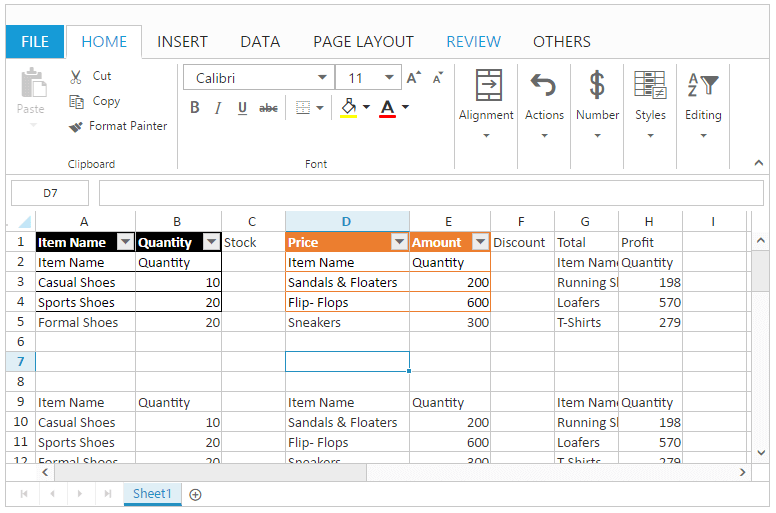
You can insert the controls like Button, Checkbox, Dropdown list and Date picker. You can use allowCellType property to enable/disable cell type operations.
To enable or disable auto rendering of cell type in the Spreadsheet use allowAutoCellType property.
To insert a Cell Type.
You can insert the cell type to the selected range of cells by one of the following ways
- Using
cellTypesproperty in sheets. - Using
addCellTypesmethod.
To remove Cell Type
You can delete the cell type in the selected range of cells by using removeCellTypes method.
The following code example describes the above behavior.
<div id="Spreadsheet"></div>$(function () {
$("#Spreadsheet").ejSpreadsheet({
// the datasource "window.defaultData" is referred from 'http://js.syncfusion.com/demos/web/scripts/xljsondata.min.js'
sheets: [{
rangeSettings: [{ dataSource: window.defaultData }],
cellTypes: [{ 'range': 'A1', 'settings': { 'type': ej.Spreadsheet.CustomCellType.DropDownList, 'dataSourceRange': 'A2:A11' } },
{ 'range': 'D1', 'settings': {"type" : ej.Spreadsheet.CustomCellType.Button, "text" : "Button1", "background-color" : "green" } }
{ 'range': 'C1', 'settings': { 'type': ej.Spreadsheet.CustomCellType.DropDownList, 'dataSourceRange': 'A2:A11' } }]
}],
allowCellType: true,
loadComplete: "loadComplete"
});
});
function loadComplete() {
var excelCellType = this.XLCellType;
if (!this.isImport) {
excelCellType.addCellTypes("B1", {"type" : ej.Spreadsheet.CustomCellType.DatePicker, 'value' : '2/12/2016'}, 1);
excelCellType.addCellTypes("E1", {"type" : ej.Spreadsheet.CustomCellType.CheckBox, "isChecked" : true }, 1);
excelCellType.removeCellTypes("C1");
}
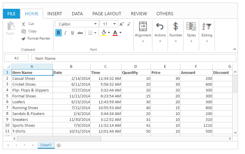
}The following output is displayed as a result of the above code example.
Chart
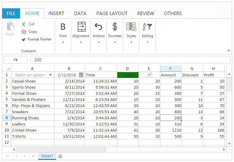
Chart is a graphical representation of data, that organizes and represents a set of numerical or qualitative data. It mostly displays the selected range of data in terms of x axis and y axis. You can use allowCharts property to enable/disable chart operations.
Types of Chart
The following types of charts are available in Spreadsheet.
- Area Chart
- Bar Chart
- Column Chart
- Line Chart
- Pie Chart
- Radar Chart
- Scatter Chart
You can create the Chart by one of the following ways,
- Using “Chart Type” button to Select the type of chart under Charts group of INSERT Tab in ribbon.
- Using
createChartmethod to create the chart.
Chart Customization
You can perform the following customizations for chart. These are available in DESIGN Tab which is enabled while clicking the chart element.
| Feature | API | Description |
|---|---|---|
| Add Chart Elements | You can add a chart element like chart axes, legends, chart title, axis title, data labels and grid lines. | |
| Switch Row/Column | You can switch the row of the chart to column of the chart and vice versa. | |
| Select Data | You can modify the data source of Chart. | |
| Chart Type | You can change the type of the chart using Chart Type dialog. | |
| Height and Width | and | You can change the height and width of the chart. |
| Chart Themes | You can change the theme of the chart. The available themes are saffron, lemon and azure in dark, light themes. | |
| Refresh Chart | To refresh the chart in the Spreadsheet. | |
| Resize Chart | To resize the chart of specified id in the Spreadsheet. |
The following code example describes the above behavior.
<div id="Spreadsheet"></div>$(function () {
$("#Spreadsheet").ejSpreadsheet({
// the datasource "window.defaultData" is referred from 'http://js.syncfusion.com/demos/web/scripts/xljsondata.min.js'
sheets: [{
rangeSettings: [{ dataSource: window.defaultData }],
}],
allowCharting: true,
loadComplete: "loadComplete"
});
});
function loadComplete() {
if (!this.isImport) {
this.XLChart.createChart("D1:E6", { type: "column", enable3D: false, marker: false, top: 40, left: 260, width: 340, height: 250 });
this.performSelection("E1");
this.XLChart.createChart("E1:F6", { type: "stackingcolumn", enable3D: false, marker: { visible: false }, top: 40, left: 620, width: 340, height: 250 });
}
}The following output is displayed as a result of the above code example.
Conditional Formatting
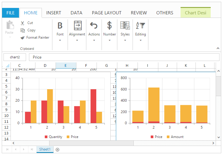
Conditional formatting helps you to apply formats to a cell or range with certain color based on the cells values. You can use allowConditionalFormats property to enable/disable Conditional formats.
Condition Definition
You can define conditions such as greater than, less than, between, equal to, text contains and date occurring for selected cells and defining value for condition. It highlights the specified cell.
You can do this by one of the following ways,
- Using “Conditional Formatting” option in Conditional Formatting button of HOME Tab in ribbon to open the conditional formatting dialog.
- Using
setCFRulemethod to define the condition. - Using
cFormatRuleinsheetsAPI. - Using
getCFRulemethod to get the defined condition.
Conditional Formatting have the following options in spreadsheet,
- Using
actionincFormatRuleAPI you can specify the conditions to apply for the range of cells in Spreadsheet. - Using
colorincFormatRuleAPI, you can specify the color to apply for the range of cell while conditional formatting. - Using
inputsincFormatRuleAPI, you can specify the inputs for conditional formatting in Spreadsheet. - Using
rangeincFormatRuleAPI, you can specify the range for conditional formatting in Spreadsheet.
The following code example describes the above behavior.
<div id="Spreadsheet"></div>$(function () {
$("#Spreadsheet").ejSpreadsheet({
// the datasource "window.defaultData" is referred from 'http://js.syncfusion.com/demos/web/scripts/xljsondata.min.js'
sheets: [{
rangeSettings: [{ dataSource: window.defaultData}],
}],
allowConditionalFormats: true,
loadComplete: "loadComplete"
});
});
function loadComplete() {
var excelFormat = this.XLCFormat;
if (!this.isImport) {
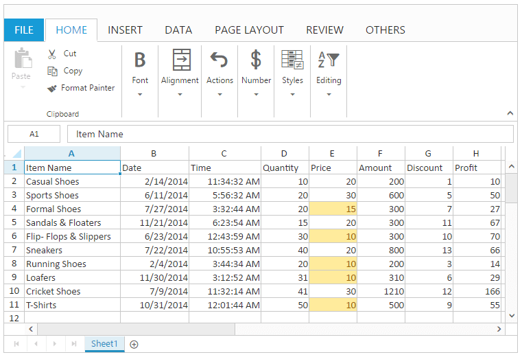
excelFormat.setCFRule({ "action": "greaterthan", "inputs": ["10"], "color": "redft", "range": "G2:G11" });
excelFormat.setCFRule({ "action": "lessthan", "inputs": ["20"], "color": "yellowft", "range": "E1:E11" });
excelFormat.setCFRule({ "action": "between", "inputs": ["300", "600"], "color": "greenft", "range": "F2:F11" });
excelFormat.setCFRule({ "action": "textcontains", "inputs": ["loafers"], "color": "redt", "range": "A1:A11" });
excelFormat.setCFRule({ "action": "dateoccur", "inputs": ["02/04/2014"], "color": "redft", "range": "B1:B11" });
excelFormat.setCFRule({ "action": "databar", "color": "redft", "range": "H1:H11" });
excelFormat.setCFRule({action: ej.Spreadsheet.CFormatRule.ColorScale, color: ej.Spreadsheet.ColorScale.GreenYellowRed, range: "D2:D11"});
}
}The following output is displayed as a result of the above code example.
Clear Rules
You can clear the defined rules by using one of the following ways,
- Using “Clear Rules” option in Conditional Formatting button of HOME Tab in ribbon to clear the rule.
- Using
clearCFmethod to clear the defined rules.
The following code example describes the above behavior.
<div id="Spreadsheet"></div>$(function () {
$("#Spreadsheet").ejSpreadsheet({
// the datasource "window.defaultData" is referred from 'http://js.syncfusion.com/demos/web/scripts/xljsondata.min.js'
sheets: [{
rangeSettings: [{ dataSource: window.defaultData}],
}],
allowConditionalFormats: true,
loadComplete: "loadComplete"
});
});
function loadComplete() {
var excelFormat = this.XLCFormat;
if (!this.isImport) {
excelFormat.setCFRule({ "action": "greaterthan", "inputs": ["10"], "color": "redft", "range": "G2:G11" });
excelFormat.setCFRule({ "action": "lessthan", "inputs": ["20"], "color": "yellowft", "range": "E1:E11" });
excelFormat.setCFRule({ "action": "between", "inputs": ["300", "600"], "color": "greenft", "range": "F2:F11" });
excelFormat.clearCF(true, "G2:G11");
excelFormat.clearCF(true, "F2:F11");
}
}The following output is displayed as a result of the above code example.
Filtering
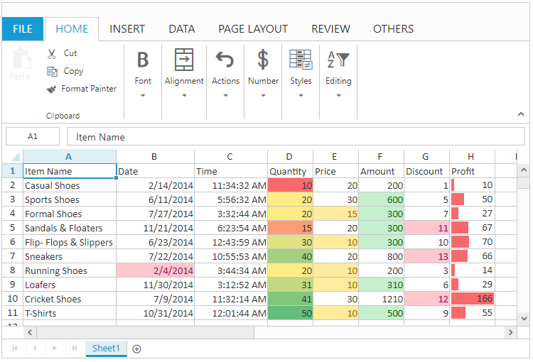
Filtering allows you to view specific rows in Spreadsheet, while hiding the other rows. When a filter is added to the header row, a drop-down menu appears in each cell of the header row. You can use allowFiltering property to enable/disable filtering.
You can apply filtering by one of the following ways,
- Using “Filter” option in Sort & Filter button under Editing group of HOME Tab in ribbon.
- Using “Filter” button under Sort and Filter group of DATA Tab in ribbon.
- Using
filtermethod.
You have following options in Filtering.
- Filter by Value.
- Filter by Color.
- Clear Filter.
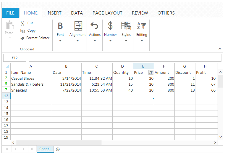
Filter by Value
You can perform filtering by using number, string. The filtered rows are only visible in the Spreadsheet. All the other rows within the filtered range were hidden.
You can do this by one of the following ways,
- Using dropdown button in filter header to open the filter dialog.
- Using context menu to select “Filter by Selected Cell’s Value” option in Filter.
- Using
filterByActiveCellmethod.
The following code example describes the above behavior.
<div id="Spreadsheet"></div>$(function () {
$("#Spreadsheet").ejSpreadsheet({
// the datasource "window.defaultData" is referred from 'http://js.syncfusion.com/demos/web/scripts/xljsondata.min.js'
sheets: [{
rangeSettings: [{ dataSource: window.defaultData }],
}],
loadComplete: "loadComplete"
});
});
function loadComplete() {
var excelFilter = this.XLFilter;
if (!this.isImport) {
this.performSelection("E2");
excelFilter.filterByActiveCell();
}
}The following output is displayed as a result of the above code example.
Filter by Color
You can perform filtering by the selected cell color or font color. The filtered rows are only visible in the Spreadsheet. You can do this by clicking “Filter by Color” option in filter dialog to select filter by cell color or font color.
NOTE
This option is only available if the selected range of cells having any color.
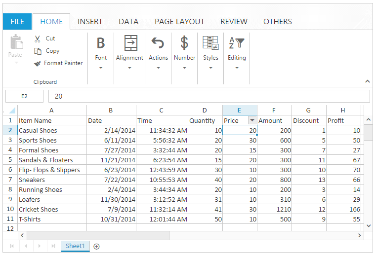
Clear Filter
You can clear the filtering to show all the filtered rows in the spreadsheet within the filtered range.
You can do this by one of the following ways,
- Using “Clear Filter” option in the filter dialog.
- Using context menu to select “Clear Filter” option in Filter.
- Using “Clear Filter” option in “Sort & Filter” button under Editing group of HOME Tab in ribbon.
- Using “Clear Filter” option under Sort and Filter group of DATA Tab in ribbon.
- Using
clearFiltermethod to perform clear filtering.
The following code example describes the above behavior.
$(function () {
    $("#Spreadsheet").ejSpreadsheet({
        // the datasource "window.defaultData" is referred from 'http://js.syncfusion.com/demos/web/scripts/xljsondata.min.js'
        sheets: [{
            rangeSettings: [{ dataSource: window.defaultData }],
        }],
        loadComplete: "loadComplete"
    });
});
function loadComplete() {
    var excelFilter = this.XLFilter;
    if (!this.isImport) {
        this.performSelection("E2");
        excelFilter.filterByActiveCell();
        excelFilter.clearFilter();
    }
}
The following output is displayed as a result of the above code example.
Picture
You can insert a picture by selecting the “Pictures” button under Illustrations group of INSERT Tab in ribbon, To enable/disable picture operations in spreadsheet use allowPictures option in pictureSettings
You can also insert a picture by usingsetPicture method.
Picture Customization
You can perform the following customizations for picture. These are available in DESIGN Tab which is enabled while clicking the picture element.
| Feature | API | Description |
|---|---|---|
| Change Picture | You can change the picture with existing picture. | |
| Reset Picture | You can reset the changes done in the picture such as border changes, height and width changes. | |
| Picture Border | You can add border to the picture. You have Border Color, Border Type and Border weight options to draw a border. | |
| Height and Width | and | You can change the height and width of the picture. |
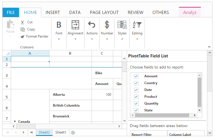
Pivot Table
Pivot table is a program tool that allows you to reorganize and summarize selected columns and rows of data to obtain a desired report. You can use enablePivotTable property to enable/disable pivot table operations.
You can do this by one of the following ways,
- Using “Pivot Table” option under Tables group of INSERT Tab in ribbon.
- Using
createPivotTablemethod to create pivot table - Using
deletePivotTablemethod to remove the pivot table.
In Pivot table we have following options,
- Using
clearPivotFieldListmethod to clear the pivot table list in Spreadsheet. - Using
refreshDataSourcemethod to refresh data in pivot table. - Using
showActivationPanelmethod to show the pivot table activationPanel in the Spreadsheet. - Using
hideActivationPanelmethod to hide the pivot table activationPanel in the Spreadsheet. - Using
apWidthmethod to define the width of the activation panel in Spreadsheet.
The following code example describes the above behavior.
<div id="Spreadsheet"></div>$(function () {
$("#Spreadsheet").ejSpreadsheet({
// the datasource "window.pivot" is referred from 'http://js.syncfusion.com/demos/web/scripts/xljsondata.min.js'
sheets: [{
rangeSettings: [{ dataSource: window.pivot }],
}],
enablePivotTable: true,
loadComplete: "loadComplete"
});
});
function loadComplete() {
if (!this.isImport) {
var settings = {
rows: [{fieldName: "Country"}, { fieldName: "State"}],
columns: [{fieldName: "Product"}],
values: [{fieldName: "Amount"},{fieldName: "Quantity"}],
filters: [{fieldName: "Date"}]
};
this.XLPivot.createPivotTable("Sheet1!$A$1:$F$25", null, null, settings);
//this.XLPivot.deletePivotTable("name");
}
}The following output is displayed as a result of the above code example.
Sorting
Sorting helps you to arrange the data to particular order in a selected range of cells. You can use allowSorting property to enable/disable sorting.
You have following options in sorting.
- Sort by Ascending or Descending.
- Sort by Color.
Sort by Ascending and Descending
You can perform number sorting by ascending or descending and string sorting by A to Z or Z to A to arrange the data.
You can do this by one of the following ways,
- By choosing “Sort A to Z” or “Sort Z to A” in Sort & Filter button under Editing group of HOME Tab in ribbon.
- Using “Sort A to Z” or “Sort Z to A” button in Sort & Filter group of DATA Tab in ribbon.
- Using context menu to select “Sort A to Z” or “Sort Z to A” for strings and option in Sort.
- Using “Sort A to Z” or “Sort Z to A” for strings an “Sort Smallest to Largest” or “Sort Largest to Smallest” for numbers in filter dialog.
- Using
sortByRangemethod.
The following code example describes the above behavior.
<div id="Spreadsheet"></div>$(function () {
$("#Spreadsheet").ejSpreadsheet({
// the datasource "window.defaultData" is referred from 'http://js.syncfusion.com/demos/web/scripts/xljsondata.min.js'
sheets: [{
rangeSettings: [{ dataSource: window.defaultData }],
}],
loadComplete: "loadComplete"
});
});
function loadComplete() {
var excelSort = this.XLSort, excelFormat = this.XLFormat;
if (!this.isImport) {
excelSort.sortByRange("A2:A10", "A", "ascending");
excelSort.sortByRange("E2:E10", "E", "descending");
}
}The following output is displayed as a result of the above code example.
Sort by Color
You can perform sort by color to arrange the data based on the selected cell’s background color or font color. This option is only available if the selected range of cells having any color.
You can do this by one of the following ways,
- Using “Sort By Color” option in filter dialog to perform sorting by cell color or font color.
- Using context menu to select “Put Selected Cell Color To The Top” or “Put Selected Font Color To The Top” in Sort option.
- Using
sortByColormethod.
Table
A table is a data structure that organizes information into rows and columns. You can use allowFormatAsTable property to enable/disable table operations.
You can do this by one of the following ways,
- Using “Format As Table” under Styles group of HOME Tab in ribbon.
- Using Table option under Tables group of INSERT Tab in ribbon.
- Using
createTablemethod to insert a table andremoveTableto delete a table. - Using
convertToRangemethod to convert table range to normal range.
Table Customization
You can perform the following customizations for table. These are available in DESIGN Tab which is enabled while clicking the table.
| Feature | Description |
|---|---|
| Resize Table | You can resize the table only to increase row count. |
| Convert to Range | You can remove the table using this option. |
| First Column | You can highlight the first column of the table. |
| Last Column | You can highlight the last column of the table. |
| Total Row | You can insert a new row in the bottom of the table to display the total value of the last column. You can toggle this by using checkbox. |
| Filter Button | You can able to hide or unhide the filter icons in the filter header of a table. |
The following code example describes the above behavior.
<div id="Spreadsheet"></div>$(function () {
$("#Spreadsheet").ejSpreadsheet({
// the datasource "window.bill" is referred from 'http://js.syncfusion.com/demos/web/scripts/xljsondata.min.js'
sheets: [{
rangeSettings: [{ dataSource: window.bill }],
}],
allowFormatAsTable: true,
loadComplete: "loadComplete"
});
});
function loadComplete() {
var excelFormat = this.XLFormat;
if (!this.isImport) {
excelFormat.createTable({ "header": true, "formatName": "TableStyleLight8" }, "A1:B4");
excelFormat.createTable({ "header": true, "formatName": "TableStyleLight10" }, "D1:E4");
}
}The following output is displayed as a result of the above code example.