Working with charts using various operations
7 Feb 202424 minutes to read
Essential XlsIO has support for creating and modifying Excel charts inside a workbook or as a chart worksheet.
Creating a Chart
The IChartShape interface represents the chart in a worksheet. A chart can be created either through the existing data in the worksheet, directly entering series or by adding series one by one.
The following code example illustrates how to create a chart through the existing data in the worksheet.
using (ExcelEngine excelEngine = new ExcelEngine())
{
  IApplication application = excelEngine.Excel;
  application.DefaultVersion = ExcelVersion.Excel2013;
  FileStream inputStream = new FileStream("Sample.xlsx", FileMode.Open, FileAccess.Read);
  IWorkbook workbook = application.Workbooks.Open(inputStream, ExcelOpenType.Automatic);
  IWorksheet sheet = workbook.Worksheets[0];

  //Create a Chart
  IChartShape chart = sheet.Charts.Add();

  //Set Chart Type
  chart.ChartType = ExcelChartType.Column_Clustered;

  //Set data range in the worksheet
  chart.DataRange = sheet.Range["A1:E5"];

  //Saving the workbook as stream
  FileStream stream = new FileStream("Chart.xlsx", FileMode.Create, FileAccess.ReadWrite);
  workbook.SaveAs(stream);
  stream.Dispose();
}
using (ExcelEngine excelEngine = new ExcelEngine())
{
IApplication application = excelEngine.Excel;
application.DefaultVersion = ExcelVersion.Excel2013;
IWorkbook workbook = application.Workbooks.Open("Sample.xlsx", ExcelOpenType.Automatic);
IWorksheet sheet = workbook.Worksheets[0];
//Create a Chart
IChartShape chart = sheet.Charts.Add();
//Set Chart Type
chart.ChartType = ExcelChartType.Column_Clustered;
//Set data range in the worksheet
chart.DataRange = sheet.Range["A1:E5"];
workbook.SaveAs("Chart.xlsx");
}Using excelEngine As ExcelEngine = New ExcelEngine()
Dim application As IApplication = excelEngine.Excel
application.DefaultVersion = ExcelVersion.Excel2013
Dim workbook As IWorkbook = application.Workbooks.Open("Sample.xlsx", ExcelOpenType.Automatic)
Dim sheet As IWorksheet = workbook.Worksheets(0)
'Create a Chart
Dim chart As IChartShape = sheet.Charts.Add()
'Set Chart Type
chart.ChartType = ExcelChartType.Column_Clustered
'Set data range in the worksheet
chart.DataRange = sheet.Range("A1:E5")
workbook.SaveAs("Chart.xlsx")
End UsingA complete working example to create a chart in C# is present on this GitHub page.
Creating a Chart from directly entered Values
A chart in XlsIO can also be created from directly entered values. The Following code snippets illustrate how to create a chart from directly entered values.
using (ExcelEngine excelEngine = new ExcelEngine())
{
  IApplication application = excelEngine.Excel;
  application.DefaultVersion = ExcelVersion.Excel2013;
  IWorkbook workbook = application.Workbooks.Create(1);
  IWorksheet sheet = workbook.Worksheets[0];

  object[] yValues = new object[] { 2000, 1000, 1000 };
  object[] xValues = new object[] { "Total Income", "Expenses", "Profit" };

  //Adding series and values
  IChartShape chart = sheet.Charts.Add();
  IChartSerie serie = chart.Series.Add(ExcelChartType.Pie);

  //Enters the X and Y values directly
  serie.EnteredDirectlyValues = yValues;
  serie.EnteredDirectlyCategoryLabels = xValues;

  //Saving the workbook as stream
  FileStream stream = new FileStream("Chart.xlsx", FileMode.Create, FileAccess.ReadWrite);
  workbook.SaveAs(stream);
  stream.Dispose();
}
using (ExcelEngine excelEngine = new ExcelEngine())
{
IApplication application = excelEngine.Excel;
application.DefaultVersion = ExcelVersion.Excel2013;
IWorkbook workbook = application.Workbooks.Create(1);
IWorksheet sheet = workbook.Worksheets[0];
object[] yValues = new object[] { 2000, 1000, 1000 };
object[] xValues = new object[] { "Total Income", "Expenses", "Profit" };
//Adding series and values
IChartShape chart = sheet.Charts.Add();
IChartSerie serie = chart.Series.Add(ExcelChartType.Pie);
//Enters the X and Y values directly
serie.EnteredDirectlyValues = yValues;
serie.EnteredDirectlyCategoryLabels = xValues;
workbook.SaveAs("Chart.xlsx");
}Using excelEngine As ExcelEngine = New ExcelEngine()
Dim application As IApplication = excelEngine.Excel
application.DefaultVersion = ExcelVersion.Excel2013
Dim workbook As IWorkbook = application.Workbooks.Create(1)
Dim sheet As IWorksheet = workbook.Worksheets(0)
Dim yValues As Object() = New Object() {2000, 1000, 1000}
Dim xValues As Object() = New Object() {"Total Income", "Expenses", "Profit"}
'Adding series and values
Dim chart As IChartShape = sheet.Charts.Add()
Dim serie As IChartSerie = chart.Series.Add(ExcelChartType.Pie)
'Enters the X and Y values directly
serie.EnteredDirectlyValues = yValues
serie.EnteredDirectlyCategoryLabels = xValues
workbook.SaveAs("Chart.xlsx")
End UsingA complete working example to create a chart from scratch in C# is present on this GitHub page.
Creating a Chart by adding Series
A chart can also be created by adding series one by one. The following code illustrates how to create a chart through series.
using (ExcelEngine excelEngine = new ExcelEngine())
{
  IApplication application = excelEngine.Excel;
  application.DefaultVersion = ExcelVersion.Excel2013;
  IWorkbook workbook = application.Workbooks.Create(1);
  IWorksheet sheet = workbook.Worksheets[0];

  //Inserts the sample data for the chart
  sheet.Range["A1"].Text = "Month";
  sheet.Range["B1"].Text = "Product A";
  sheet.Range["C1"].Text = "Product B";

  //Months
  sheet.Range["A2"].Text = "Jan";
  sheet.Range["A3"].Text = "Feb";
  sheet.Range["A4"].Text = "Mar";
  sheet.Range["A5"].Text = "Apr";
  sheet.Range["A6"].Text = "May";

  //Create a random Data
  Random r = new Random();
  for (int i = 2; i <= 6; i++)
  {
	for (int j = 2; j <= 3; j++)
	{
      sheet.Range[i, j].Number = r.Next(0, 500);
	}
  }
  IChartShape chart = sheet.Charts.Add();

  //Set chart type
  chart.ChartType = ExcelChartType.Line;

  //Set Chart Title
  chart.ChartTitle = "Product Sales comparison";

  //Set first serie
  IChartSerie productA = chart.Series.Add("ProductA");
  productA.Values = sheet.Range["B2:B6"];
  productA.CategoryLabels = sheet.Range["A2:A6"];

  //Set second serie
  IChartSerie productB = chart.Series.Add("ProductB");
  productB.Values = sheet.Range["C2:C6"];
  productB.CategoryLabels = sheet.Range["A2:A6"];

  //Saving the workbook as stream
  FileStream stream = new FileStream("Chart.xlsx", FileMode.Create, FileAccess.ReadWrite);
  workbook.SaveAs(stream);
  stream.Dispose();
}
using (ExcelEngine excelEngine = new ExcelEngine())
{
IApplication application = excelEngine.Excel;
application.DefaultVersion = ExcelVersion.Excel2013;
IWorkbook workbook = application.Workbooks.Create(1);
IWorksheet sheet = workbook.Worksheets[0];
//Inserts the sample data for the chart
sheet.Range["A1"].Text = "Month";
sheet.Range["B1"].Text = "Product A";
sheet.Range["C1"].Text = "Product B";
//Months
sheet.Range["A2"].Text = "Jan";
sheet.Range["A3"].Text = "Feb";
sheet.Range["A4"].Text = "Mar";
sheet.Range["A5"].Text = "Apr";
sheet.Range["A6"].Text = "May";
//Create a random Data
Random r = new Random();
for (int i = 2; i <= 6; i++)
{
for (int j = 2; j <= 3; j++)
{
sheet.Range[i, j].Number = r.Next(0, 500);
}
}
IChartShape chart = sheet.Charts.Add();
//Set chart type
chart.ChartType = ExcelChartType.Line;
//Set Chart Title
chart.ChartTitle = "Product Sales comparison";
//Set first serie
IChartSerie productA = chart.Series.Add("ProductA");
productA.Values = sheet.Range["B2:B6"];
productA.CategoryLabels = sheet.Range["A2:A6"];
//Set second serie
IChartSerie productB = chart.Series.Add("ProductB");
productB.Values = sheet.Range["C2:C6"];
productB.CategoryLabels = sheet.Range["A2:A6"];
workbook.SaveAs("Chart.xlsx");
}A complete working example to create a chart through series in C# is present on this GitHub page.
Creating a chart Sheet
The following code snippet shows how to create a chart sheet (separate sheet).
using (ExcelEngine excelEngine = new ExcelEngine())
{
  IApplication application = excelEngine.Excel;
  application.DefaultVersion = ExcelVersion.Excel2013;
  FileStream inputStream = new FileStream("Sample.xlsx", FileMode.Open, FileAccess.Read);
  IWorkbook workbook = application.Workbooks.Open(inputStream, ExcelOpenType.Automatic);
  IWorksheet sheet = workbook.Worksheets[0];

  //Add the chart sheet
  IChart chart = workbook.Charts.Add();
  chart.ChartType = ExcelChartType.Column_Clustered;
  chart.DataRange = sheet.Range["A1:E5"];

  //Saving the workbook as stream
  FileStream stream = new FileStream("Chart.xlsx", FileMode.Create, FileAccess.ReadWrite);
  workbook.SaveAs(stream);
  stream.Dispose();
}
using (ExcelEngine excelEngine = new ExcelEngine())
{
IApplication application = excelEngine.Excel;
application.DefaultVersion = ExcelVersion.Excel2013;
IWorkbook workbook = application.Workbooks.Open("Sample.xlsx", ExcelOpenType.Automatic);
IWorksheet sheet = workbook.Worksheets[0];
//Add the chart sheet
IChart chart = workbook.Charts.Add();
chart.ChartType = ExcelChartType.Column_Clustered;
chart.DataRange = sheet.Range["A1:E5"];
workbook.SaveAs("Chart.xlsx");
}Using excelEngine As ExcelEngine = New ExcelEngine()
Dim application As IApplication = excelEngine.Excel
application.DefaultVersion = ExcelVersion.Excel2013
Dim workbook As IWorkbook = application.Workbooks.Open("Sample.xlsx", ExcelOpenType.Automatic)
Dim sheet As IWorksheet = workbook.Worksheets(0)
'Add the chart sheet
Dim chart As IChart = workbook.Charts.Add()
chart.ChartType = ExcelChartType.Column_Clustered
chart.DataRange = sheet.Range("A1:E5")
workbook.SaveAs("Chart.xlsx")
End UsingA complete working example to create a chart worksheet in C# is present on this GitHub page.
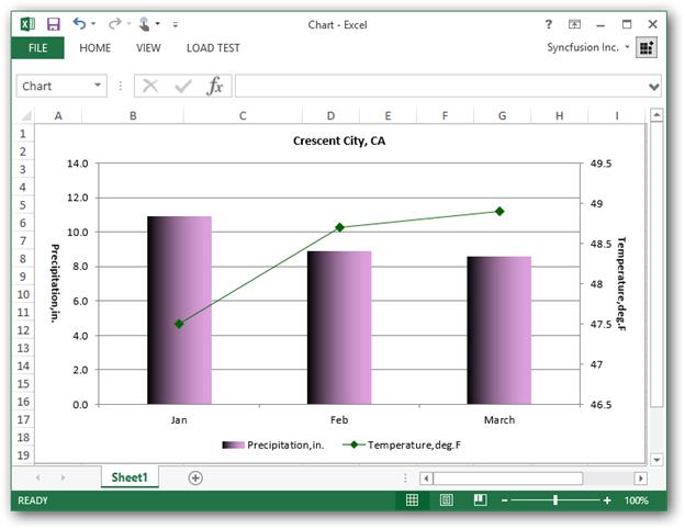
Creating Custom Charts
A custom chart can be created by using different types of charts for different data series.
For example, you can use a column chart for the first data series and a line chart for the second series. As a result you will have a column chart, combined with a line chart.
This sample also explains different chart properties like
Set Data Range to Chart
//Add a new chart with data range
IChartShape chart = sheet.Charts.Add();
chart.DataRange = sheet.Range["A3:C6"];
//Add a new chart with data range
IChartShape chart = sheet.Charts.Add();
chart.DataRange = sheet.Range["A3:C6"];'Add a new chart with data range
Dim chart As IChartShape = sheet.Charts.Add()
chart.DataRange = sheet.Range("A3:C6")Name the Chart and Set Chart Title
//Set chart name and chart title
chart.Name = "CrescentCity,CA";
chart.ChartTitle = "Crescent City, CA";//Set chart name and chart title
chart.Name = "CrescentCity,CA";
chart.ChartTitle = "Crescent City, CA";'Set chart name and chart title
chart.Name = "CrescentCity,CA"
chart.ChartTitle = "Crescent City, CA"Different Primary Value Axis Properties
//Axis title
chart.PrimaryValueAxis.Title = "Precipitation,in.";
//Axis title area text angle rotation
chart.PrimaryValueAxis.TitleArea.TextRotationAngle = 90;
//Maximum value in the axis
chart.PrimaryValueAxis.MaximumValue = 14.0;
//Number format for axis
chart.PrimaryValueAxis.NumberFormat = "0.0";
//Display unit for axis
chart.PrimaryValueAxis.DisplayUnit = ExcelChartDisplayUnit.Hundreds;//Axis title
chart.PrimaryValueAxis.Title = "Precipitation,in.";
//Axis title area text angle rotation
chart.PrimaryValueAxis.TitleArea.TextRotationAngle = 90;
//Maximum value in the axis
chart.PrimaryValueAxis.MaximumValue = 14.0;
//Number format for axis
chart.PrimaryValueAxis.NumberFormat = "0.0";
//Display unit for axis
chart.PrimaryValueAxis.DisplayUnit = ExcelChartDisplayUnit.Hundreds;'Axis title
chart.PrimaryValueAxis.Title = "Precipitation,in."
'Axis title area text angle rotation
chart.PrimaryValueAxis.TitleArea.TextRotationAngle = 90
'Maximum value in the axis
chart.PrimaryValueAxis.MaximumValue = 14.0
'Number format for axis
chart.PrimaryValueAxis.NumberFormat = "0.0"
'Display unit for axis
chart.PrimaryValueAxis.DisplayUnit = ExcelChartDisplayUnit.HundredsDifferent Secondary Value Axis Properties
//MaxCross in axis
chart.SecondaryValueAxis.IsMaxCross = true;
//Axis title
chart.SecondaryValueAxis.Title = "Temperature,deg.F";
//Axis title area text angle rotation
chart.SecondaryValueAxis.TitleArea.TextRotationAngle = 90;//MaxCross in axis
chart.SecondaryValueAxis.IsMaxCross = true;
//Axis title
chart.SecondaryValueAxis.Title = "Temperature,deg.F";
//Axis title area text angle rotation
chart.SecondaryValueAxis.TitleArea.TextRotationAngle = 90;'MaxCross in axis
chart.SecondaryValueAxis.IsMaxCross = true
'Axis title
chart.SecondaryValueAxis.Title = "Temperature,deg.F"
'Axis title area text angle rotation
chart.SecondaryValueAxis.TitleArea.TextRotationAngle = 90Different Secondary Category Axis Properties
//MaxCross in axis
chart.SecondaryCategoryAxis.IsMaxCross = true;
//Select border line color
chart.SecondaryCategoryAxis.Border.LineColor = Color.Transparent;
//Select major tick mark option
chart.SecondaryCategoryAxis.MajorTickMark = ExcelTickMark.TickMark_None;
//Select tick label position
chart.SecondaryCategoryAxis.TickLabelPosition = ExcelTickLabelPosition.TickLabelPosition_None;//MaxCross in axis
chart.SecondaryCategoryAxis.IsMaxCross = true;
//Select border line color
chart.SecondaryCategoryAxis.Border.LineColor = Color.Transparent;
//Select major tick mark option
chart.SecondaryCategoryAxis.MajorTickMark = ExcelTickMark.TickMark_None;
//Select tick label position
chart.SecondaryCategoryAxis.TickLabelPosition = ExcelTickLabelPosition.TickLabelPosition_None;'MaxCross in axis
chart.SecondaryCategoryAxis.IsMaxCross = true
'Select border line color
chart.SecondaryCategoryAxis.Border.LineColor = Color.Transparent
'Select major tick mark option
chart.SecondaryCategoryAxis.MajorTickMark = ExcelTickMark.TickMark_None
'Select tick label position
chart.SecondaryCategoryAxis.TickLabelPosition = ExcelTickLabelPosition.TickLabelPosition_NoneDifferent Chart Series Fill Properties
IChartSerie serieOne = chart.Series[0];
//Series name
serieOne.Name = "Precipitation,in.";
//Series fill type
serieOne.SerieFormat.Fill.FillType = ExcelFillType.Gradient;
//Series two color gradient
serieOne.SerieFormat.Fill.TwoColorGradient(ExcelGradientStyle.Vertical, ExcelGradientVariants.ShadingVariants_2);
//Series gradient color type
serieOne.SerieFormat.Fill.GradientColorType = ExcelGradientColor.TwoColor;
//Series fore color
serieOne.SerieFormat.Fill.ForeColor = Color.Plum;IChartSerie serieOne = chart.Series[0];
//Series name
serieOne.Name = "Precipitation,in.";
//Series fill type
serieOne.SerieFormat.Fill.FillType = ExcelFillType.Gradient;
//Series two color gradient
serieOne.SerieFormat.Fill.TwoColorGradient(ExcelGradientStyle.Vertical, ExcelGradientVariants.ShadingVariants_2);
//Series gradient color type
serieOne.SerieFormat.Fill.GradientColorType = ExcelGradientColor.TwoColor;
//Series fore color
serieOne.SerieFormat.Fill.ForeColor = Color.Plum;Dim serieOne As IChartSerie = chart.Series(0)
'Series name
serieOne.Name = "Precipitation,in."
'Series fill type
serieOne.SerieFormat.Fill.FillType = ExcelFillType.Gradient
'Series two color gradient
serieOne.SerieFormat.Fill.TwoColorGradient(ExcelGradientStyle.Vertical, ExcelGradientVariants.ShadingVariants_2)
'Series gradient color type
serieOne.SerieFormat.Fill.GradientColorType = ExcelGradientColor.TwoColor
'Series fore color
serieOne.SerieFormat.Fill.ForeColor = Color.PlumDifferent Marker Properties
IChartSerie serieTwo = chart.Series[1];
//Marker style
serieTwo.SerieFormat.MarkerStyle = ExcelChartMarkerType.Diamond;
//Marker size
serieTwo.SerieFormat.MarkerSize = 8;
//Marker background color
serieTwo.SerieFormat.MarkerBackgroundColor = Color.DarkGreen;
//Marker foreground color
serieTwo.SerieFormat.MarkerForegroundColor = Color.DarkGreen;IChartSerie serieTwo = chart.Series[1];
//Marker style
serieTwo.SerieFormat.MarkerStyle = ExcelChartMarkerType.Diamond;
//Marker size
serieTwo.SerieFormat.MarkerSize = 8;
//Marker background color
serieTwo.SerieFormat.MarkerBackgroundColor = Color.DarkGreen;
//Marker foreground color
serieTwo.SerieFormat.MarkerForegroundColor = Color.DarkGreen;Dim serieTwo As IChartSerie = chart.Series(1)
'Marker style
serieTwo.SerieFormat.MarkerStyle = ExcelChartMarkerType.Diamond
'Marker size
serieTwo.SerieFormat.MarkerSize = 8
'Marker background color
serieTwo.SerieFormat.MarkerBackgroundColor = Color.DarkGreen
'Marker foreground color
serieTwo.SerieFormat.MarkerForegroundColor = Color.DarkGreenDifferent Legend Properties
//Legend without overlapping the chart
chart.Legend.IncludeInLayout = true;
//Legend position
chart.Legend.Position = ExcelLegendPosition.Bottom;
//View legend horizontally
chart.Legend.IsVerticalLegend = false;//Legend without overlapping the chart
chart.Legend.IncludeInLayout = true;
//Legend position
chart.Legend.Position = ExcelLegendPosition.Bottom;
//View legend horizontally
chart.Legend.IsVerticalLegend = false;'Legend without overlapping the chart
chart.Legend.IncludeInLayout = true
'Legend position
chart.Legend.Position = ExcelLegendPosition.Bottom
'View legend horizontally
chart.Legend.IsVerticalLegend = falseThe complete code snippet illustrating the above options along with creating custom charts is shown below.
using (ExcelEngine excelEngine = new ExcelEngine())
{
IApplication application = excelEngine.Excel;
application.DefaultVersion = ExcelVersion.Excel2013;
IWorkbook workbook = application.Workbooks.Create(1);
IWorksheet sheet = workbook.Worksheets[0];
//Merge cells
sheet.Range["A1:D1"].Merge();
//Set Font style as bold
sheet.Range["A1"].CellStyle.Font.Bold = true;
//Insert data for the chart
sheet.Range["A1"].Text = "Crescent City, CA";
sheet.Range["B3"].Text = "Precipitation,in.";
sheet.Range["C3"].Text = "Temperature,deg.F";
sheet.Range["A4"].Text = "Jan";
sheet.Range["A5"].Text = "Feb";
sheet.Range["A6"].Text = "March";
sheet.Range["B4"].Number = 10.9;
sheet.Range["B5"].Number = 8.9;
sheet.Range["B6"].Number = 8.6;
sheet.Range["C4"].Number = 47.5;
sheet.Range["C5"].Number = 48.7;
sheet.Range["C6"].Number = 48.9;
//Adjust column width in used range
sheet.UsedRange.AutofitColumns();
//Add a new chart with data range
IChartShape chart = sheet.Charts.Add();
chart.DataRange = sheet.Range["A3:C6"];
//Set chart name and chart title
chart.Name = "CrescentCity,CA";
chart.ChartTitle = "Crescent City, CA";
chart.IsSeriesInRows = false;
//Set primary value axis properties
chart.PrimaryValueAxis.Title = "Precipitation,in.";
chart.PrimaryValueAxis.TitleArea.TextRotationAngle = 90;
chart.PrimaryValueAxis.MaximumValue = 14.0;
chart.PrimaryValueAxis.NumberFormat = "0.0";
//Format first serie fill properties
IChartSerie serieOne = chart.Series[0];
serieOne.Name = "Precipitation,in.";
serieOne.SerieFormat.Fill.FillType = ExcelFillType.Gradient;
serieOne.SerieFormat.Fill.TwoColorGradient(ExcelGradientStyle.Vertical, ExcelGradientVariants.ShadingVariants_2);
serieOne.SerieFormat.Fill.GradientColorType = ExcelGradientColor.TwoColor;
serieOne.SerieFormat.Fill.ForeColor = Color.Plum;
//Format second serie properties
IChartSerie serieTwo = chart.Series[1];
serieTwo.SerieType = ExcelChartType.Line_Markers;
serieTwo.Name = "Temperature,deg.F";
//Format marker properties
serieTwo.SerieFormat.MarkerStyle = ExcelChartMarkerType.Diamond;
serieTwo.SerieFormat.MarkerSize = 8;
serieTwo.SerieFormat.MarkerBackgroundColor = Color.DarkGreen;
serieTwo.SerieFormat.MarkerForegroundColor = Color.DarkGreen;
serieTwo.SerieFormat.LineProperties.LineColor = Color.DarkGreen;
//Use Secondary Axis
serieTwo.UsePrimaryAxis = false;
//MaxCross for secondary axes
chart.SecondaryCategoryAxis.IsMaxCross = true;
chart.SecondaryValueAxis.IsMaxCross = true;
//Set title for secondary value axis
chart.SecondaryValueAxis.Title = "Temperature,deg.F";
chart.SecondaryValueAxis.TitleArea.TextRotationAngle = 90;
//Set secondary category axis properties
chart.SecondaryCategoryAxis.Border.LineColor = Color.Transparent;
chart.SecondaryCategoryAxis.MajorTickMark = ExcelTickMark.TickMark_None;
chart.SecondaryCategoryAxis.TickLabelPosition = ExcelTickLabelPosition.TickLabelPosition_None;
//Set legend properties
chart.Legend.Position = ExcelLegendPosition.Bottom;
chart.Legend.IsVerticalLegend = false;
//Saving the workbook as stream
FileStream stream = new FileStream("Chart.xlsx", FileMode.Create, FileAccess.ReadWrite);
workbook.SaveAs(stream);
stream.Dispose();
}using (ExcelEngine excelEngine = new ExcelEngine())
{
IApplication application = excelEngine.Excel;
application.DefaultVersion = ExcelVersion.Excel2013;
IWorkbook workbook = application.Workbooks.Create(1);
IWorksheet sheet = workbook.Worksheets[0];
//Merge cells
sheet.Range["A1:D1"].Merge();
//Set Font style as bold
sheet.Range["A1"].CellStyle.Font.Bold = true;
//Insert data for the chart
sheet.Range["A1"].Text = "Crescent City, CA";
sheet.Range["B3"].Text = "Precipitation,in.";
sheet.Range["C3"].Text = "Temperature,deg.F";
sheet.Range["A4"].Text = "Jan";
sheet.Range["A5"].Text = "Feb";
sheet.Range["A6"].Text = "March";
sheet.Range["B4"].Number = 10.9;
sheet.Range["B5"].Number = 8.9;
sheet.Range["B6"].Number = 8.6;
sheet.Range["C4"].Number = 47.5;
sheet.Range["C5"].Number = 48.7;
sheet.Range["C6"].Number = 48.9;
//Adjust column width in used range
sheet.UsedRange.AutofitColumns();
//Add a new chart with data range
IChartShape chart = sheet.Charts.Add();
chart.DataRange = sheet.Range["A3:C6"];
//Set chart name and chart title
chart.Name = "CrescentCity,CA";
chart.ChartTitle = "Crescent City, CA";
chart.IsSeriesInRows = false;
//Set primary value axis properties
chart.PrimaryValueAxis.Title = "Precipitation,in.";
chart.PrimaryValueAxis.TitleArea.TextRotationAngle = 90;
chart.PrimaryValueAxis.MaximumValue = 14.0;
chart.PrimaryValueAxis.NumberFormat = "0.0";
//Format first serie fill properties
IChartSerie serieOne = chart.Series[0];
serieOne.Name = "Precipitation,in.";
serieOne.SerieFormat.Fill.FillType = ExcelFillType.Gradient;
serieOne.SerieFormat.Fill.TwoColorGradient(ExcelGradientStyle.Vertical, ExcelGradientVariants.ShadingVariants_2);
serieOne.SerieFormat.Fill.GradientColorType = ExcelGradientColor.TwoColor;
serieOne.SerieFormat.Fill.ForeColor = Color.Plum;
//Format second serie properties
IChartSerie serieTwo = chart.Series[1];
serieTwo.SerieType = ExcelChartType.Line_Markers;
serieTwo.Name = "Temperature,deg.F";
//Format marker properties
serieTwo.SerieFormat.MarkerStyle = ExcelChartMarkerType.Diamond;
serieTwo.SerieFormat.MarkerSize = 8;
serieTwo.SerieFormat.MarkerBackgroundColor = Color.DarkGreen;
serieTwo.SerieFormat.MarkerForegroundColor = Color.DarkGreen;
serieTwo.SerieFormat.LineProperties.LineColor = Color.DarkGreen;
//Use Secondary Axis
serieTwo.UsePrimaryAxis = false;
//MaxCross for secondary axes
chart.SecondaryCategoryAxis.IsMaxCross = true;
chart.SecondaryValueAxis.IsMaxCross = true;
//Set title for secondary value axis
chart.SecondaryValueAxis.Title = "Temperature,deg.F";
chart.SecondaryValueAxis.TitleArea.TextRotationAngle = 90;
//Set secondary category axis properties
chart.SecondaryCategoryAxis.Border.LineColor = Color.Transparent;
chart.SecondaryCategoryAxis.MajorTickMark = ExcelTickMark.TickMark_None;
chart.SecondaryCategoryAxis.TickLabelPosition = ExcelTickLabelPosition.TickLabelPosition_None;
//Set legend properties
chart.Legend.Position = ExcelLegendPosition.Bottom;
chart.Legend.IsVerticalLegend = false;
workbook.SaveAs("Chart.xlsx");
}Dim excelEngine As New ExcelEngine()
Using excelEngine As ExcelEngine = New ExcelEngine()
Dim application As IApplication = excelEngine.Excel
application.DefaultVersion = ExcelVersion.Excel2013
Dim workbook As IWorkbook = application.Workbooks.Create(1)
Dim sheet As IWorksheet = workbook.Worksheets(0)
'Merge cells
sheet.Range("A1:D1").Merge()
'Set Font style as bold
sheet.Range("A1").CellStyle.Font.Bold = True
'Insert data for the chart
sheet.Range("A1").Text = "Crescent City, CA"
sheet.Range("B3").Text = "Precipitation,in."
sheet.Range("C3").Text = "Temperature,deg.F"
sheet.Range("A4").Text = "Jan"
sheet.Range("A5").Text = "Feb"
sheet.Range("A6").Text = "March"
sheet.Range("B4").Number = 10.9
sheet.Range("B5").Number = 8.9
sheet.Range("B6").Number = 8.6
sheet.Range("C4").Number = 47.5
sheet.Range("C5").Number = 48.7
sheet.Range("C6").Number = 48.9
'Adjust column width in used range
sheet.UsedRange.AutofitColumns()
'Add a new chart with data range
Dim chart As IChartShape = sheet.Charts.Add()
chart.DataRange = sheet.Range("A3:C6")
'Set chart name and chart title
chart.Name = "CrescentCity,CA"
chart.ChartTitle = "Crescent City, CA"
chart.IsSeriesInRows = False
'Set primary value axis properties
chart.PrimaryValueAxis.Title = "Precipitation,in."
chart.PrimaryValueAxis.TitleArea.TextRotationAngle = 90
chart.PrimaryValueAxis.MaximumValue = 14.0
chart.PrimaryValueAxis.NumberFormat = "0.0"
'Format first serie fill properties
Dim serieOne As IChartSerie = chart.Series(0)
serieOne.Name = "Precipitation,in."
serieOne.SerieFormat.Fill.FillType = ExcelFillType.Gradient
serieOne.SerieFormat.Fill.TwoColorGradient(ExcelGradientStyle.Vertical, ExcelGradientVariants.ShadingVariants_2)
serieOne.SerieFormat.Fill.GradientColorType = ExcelGradientColor.TwoColor
serieOne.SerieFormat.Fill.ForeColor = Color.Plum
'Format second serie properties
Dim serieTwo As IChartSerie = chart.Series(1)
serieTwo.SerieType = ExcelChartType.Line_Markers
serieTwo.Name = "Temperature,deg.F"
'Format marker properties
serieTwo.SerieFormat.MarkerStyle = ExcelChartMarkerType.Diamond
serieTwo.SerieFormat.MarkerSize = 8
serieTwo.SerieFormat.MarkerBackgroundColor = Color.DarkGreen
serieTwo.SerieFormat.MarkerForegroundColor = Color.DarkGreen
serieTwo.SerieFormat.LineProperties.LineColor = Color.DarkGreen
'Use Secondary Axis
serieTwo.UsePrimaryAxis = False
'MaxCross for secondary axes
chart.SecondaryCategoryAxis.IsMaxCross = True
chart.SecondaryValueAxis.IsMaxCross = True
'Set title for secondary value axis
chart.SecondaryValueAxis.Title = "Temperature,deg.F"
chart.SecondaryValueAxis.TitleArea.TextRotationAngle = 90
'Set secondary category axis properties
chart.SecondaryCategoryAxis.Border.LineColor = Color.Transparent
chart.SecondaryCategoryAxis.MajorTickMark = ExcelTickMark.TickMark_None
chart.SecondaryCategoryAxis.TickLabelPosition = ExcelTickLabelPosition.TickLabelPosition_None
'Set legend properties
chart.Legend.Position = ExcelLegendPosition.Bottom
chart.Legend.IsVerticalLegend = False
workbook.SaveAs("Chart.xlsx")
End UsingA complete working example to create a custom chart in C# is present on this GitHub page.
Remove a chart
The following code snippet shows how to remove the chart from the worksheet using Remove method.
using (ExcelEngine excelEngine = new ExcelEngine())
{
  IApplication application = excelEngine.Excel;
  application.DefaultVersion = ExcelVersion.Excel2013;
  FileStream inputStream = new FileStream("Sample.xlsx", FileMode.Open, FileAccess.Read);
  IWorkbook workbook = application.Workbooks.Open(inputStream, ExcelOpenType.Automatic);
  IWorksheet sheet = workbook.Worksheets[0];
  IChartShape chart = sheet.Charts[0];

  //Remove the chart from the worksheet
  chart.Remove();

  //Saving the workbook as stream
  FileStream stream = new FileStream("Chart.xlsx", FileMode.Create, FileAccess.ReadWrite);
  workbook.SaveAs(stream);
  stream.Dispose();
}
using (ExcelEngine excelEngine = new ExcelEngine())
{
IApplication application = excelEngine.Excel;
application.DefaultVersion = ExcelVersion.Excel2013;
IWorkbook workbook = application.Workbooks.Open("Sample.xlsx", ExcelOpenType.Automatic);
IWorksheet sheet = workbook.Worksheets[0];
IChartShape chart = sheet.Charts[0];
//Remove the chart from the worksheet
chart.Remove();
workbook.SaveAs("Chart.xlsx");
}Using excelEngine As ExcelEngine = New ExcelEngine()
Dim application As IApplication = excelEngine.Excel
application.DefaultVersion = ExcelVersion.Excel2013
Dim workbook As IWorkbook = application.Workbooks.Open("Sample.xlsx", ExcelOpenType.Automatic)
Dim sheet As IWorksheet = workbook.Worksheets(0)
Dim chart As IChartShape = sheet.Charts(0)
'Remove the chart from the worksheet
chart.Remove()
workbook.SaveAs("Chart.xlsx")
End UsingA complete working example to remove chart in C# is present on this GitHub page.
Chart Appearance Settings
The appearance of a chart can be modified according to the convenience and usage.
Elements of Chart
The following screen shot shows the elements of chart.
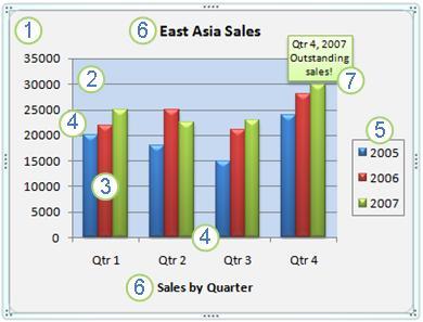
- The chart area of the chart.
- The plot area of the chart.
- The data points of the data series that are plotted in the chart.
- The horizontal (category) and vertical (value) axis along which the data is plotted in the chart.
- The legend of the chart.
- A chart axis title that you can use in the chart.
- A data label that you can use to identify the details of a data point in a data series.
Chart Area Appearance
The following code snippet shows how to modify the appearance of the chart area.
//Format Chart Area
IChartFrameFormat chartArea = chart.ChartArea;

//Chart Area Settings
chartArea.Fill.FillType = ExcelFillType.Gradient;

//Set Fill Effects
chartArea.Fill.BackColor = Color.FromArgb(205, 217, 234);
chartArea.Fill.ForeColor = Color.White;
//Format Chart Area
IChartFrameFormat chartArea = chart.ChartArea;
//Chart Area Settings
chartArea.Fill.FillType = ExcelFillType.Gradient;
//Set Fill Effects
chartArea.Fill.BackColor = Color.FromArgb(205, 217, 234);
chartArea.Fill.ForeColor = Color.White;'Format Chart Area
Dim chartArea As IChartFrameFormat = chart.ChartArea
'Chart Area Settings
chartArea.Fill.FillType = ExcelFillType.Gradient
'Set Fill Effects
chartArea.Fill.BackColor = Color.FromArgb(205, 217, 234)
chartArea.Fill.ForeColor = Color.WhitePlot Area Appearance
The following code snippet shows how to modify the appearance of the plot area.
//Set Plot Area
IChartFrameFormat chartPlotArea = chart.PlotArea;

//Set fill color
chartPlotArea.Fill.BackColor = Color.FromArgb(205, 217, 234);
chartPlotArea.Fill.ForeColor = Color.White;
//Set Plot Area
IChartFrameFormat chartPlotArea = chart.PlotArea;
//Set fill color
chartPlotArea.Fill.BackColor = Color.FromArgb(205, 217, 234);
chartPlotArea.Fill.ForeColor = Color.White;'Set Plot Area
Dim chartPlotArea As IChartFrameFormat = chart.PlotArea
'Set fill color
chartPlotArea.Fill.BackColor = Color.FromArgb(205, 217, 234)
chartPlotArea.Fill.ForeColor = Color.WhiteData Labels Appearance
The following code snippet illustrates how to modify the appearance of data labels.
IChartSerie serie =  chart.Series[0];

//Set data labels color
serie.DataPoints.DefaultDataPoint.DataLabels.Color = ExcelKnownColors.Blue;
serie.DataPoints.DefaultDataPoint.DataLabels.IsValue = true;
IChartSerie serie = chart.Series[0];
//Set data labels color
serie.DataPoints.DefaultDataPoint.DataLabels.Color = ExcelKnownColors.Blue;
serie.DataPoints.DefaultDataPoint.DataLabels.IsValue = true;Dim serie As IChartSerie = chart.Series(0)
'Set data labels color
serie.DataPoints.DefaultDataPoint.DataLabels.Color = ExcelKnownColors.Blue
serie.DataPoints.DefaultDataPoint.DataLabels.IsValue = TrueSeries Appearance
The following code snippet illustrates how to modify the appearance of chart series.
IChartSerie serie = chart.Series[0];

//Fill Effects
serie.SerieFormat.Fill.FillType = ExcelFillType.Gradient;
serie.SerieFormat.Fill.ForeColor = Color.Yellow;
IChartSerie serie = chart.Series[0];
//Fill Effects
serie.SerieFormat.Fill.FillType = ExcelFillType.Gradient;
serie.SerieFormat.Fill.ForeColor = Color.Yellow;Dim serie As IChartSerie = chart.Series(0)
'Fill Effects
serie.SerieFormat.Fill.FillType = ExcelFillType.Gradient
serie.SerieFormat.Fill.ForeColor = Color.YellowThe complete code snippet illustrating the above options is shown below.
using (ExcelEngine excelEngine = new ExcelEngine())
{
  IApplication application = excelEngine.Excel;
  application.DefaultVersion = ExcelVersion.Excel2013;
  FileStream inputStream = new FileStream("Sample.xlsx", FileMode.Open, FileAccess.Read);
  IWorkbook workbook = application.Workbooks.Open(inputStream, ExcelOpenType.Automatic);
  IWorksheet sheet = workbook.Worksheets[0];

  IChartShape chart = sheet.Charts.Add();
  chart.DataRange = sheet.UsedRange;

  //Format Chart Area
  IChartFrameFormat chartArea = chart.ChartArea;
  //Fill Effects
  chartArea.Fill.FillType = ExcelFillType.Gradient;

  //Set chart area fill color
  chartArea.Fill.BackColor = Color.FromArgb(205, 217, 234);
  chartArea.Fill.ForeColor = Color.WhiteSmoke;

  //Format Plot Area
  IChartFrameFormat chartPlotArea = chart.PlotArea;
  //Fill Effects
  chartPlotArea.Fill.FillType = ExcelFillType.Gradient;

  //Set plot area fill color
  chartPlotArea.Fill.BackColor = Color.FromArgb(205, 217, 234);
  chartPlotArea.Fill.ForeColor = Color.YellowGreen;

  //Saving the workbook as stream
  FileStream stream = new FileStream("Chart.xlsx", FileMode.Create, FileAccess.ReadWrite);
  workbook.SaveAs(stream);
  stream.Dispose();
}
using (ExcelEngine excelEngine = new ExcelEngine())
{
IApplication application = excelEngine.Excel;
application.DefaultVersion = ExcelVersion.Excel2013;
IWorkbook workbook = application.Workbooks.Open("Sample.xlsx", ExcelOpenType.Automatic);
IWorksheet sheet = workbook.Worksheets[0];
IChartShape chart = sheet.Charts.Add();
chart.DataRange = sheet.UsedRange;
//Format Chart Area
IChartFrameFormat chartArea = chart.ChartArea;
//Fill Effects
chartArea.Fill.FillType = ExcelFillType.Gradient;
//Set chart area fill color
chartArea.Fill.BackColor = Color.FromArgb(205, 217, 234);
chartArea.Fill.ForeColor = Color.WhiteSmoke;
//Format Plot Area
IChartFrameFormat chartPlotArea = chart.PlotArea;
//Fill Effects
chartPlotArea.Fill.FillType = ExcelFillType.Gradient;
//Set plot area fill color
chartPlotArea.Fill.BackColor = Color.FromArgb(205, 217, 234);
chartPlotArea.Fill.ForeColor = Color.YellowGreen;
workbook.SaveAs("Chart.xlsx");
}Using excelEngine As ExcelEngine = New ExcelEngine()
Dim application As IApplication = excelEngine.Excel
application.DefaultVersion = ExcelVersion.Excel2013
Dim workbook As IWorkbook = application.Workbooks.Open("Sample.xlsx", ExcelOpenType.Automatic)
Dim sheet As IWorksheet = workbook.Worksheets(0)
Dim chart As IChartShape = sheet.Charts.Add()
chart.DataRange = sheet.UsedRange
'Format Chart Area
Dim chartArea As IChartFrameFormat = chart.ChartArea
'Fill Effects
chartArea.Fill.FillType = ExcelFillType.Gradient
'Set chart area fill color
chartArea.Fill.BackColor = Color.FromArgb(205, 217, 234)
chartArea.Fill.ForeColor = Color.White
'Format Plot Area
Dim chartPlotArea As IChartFrameFormat = chart.PlotArea
'Fill Effects
chartPlotArea.Fill.FillType = ExcelFillType.Gradient
'Set plot area fill color
chartPlotArea.Fill.BackColor = Color.FromArgb(205, 217, 234)
chartPlotArea.Fill.ForeColor = Color.White
workbook.SaveAs("Chart.xlsx")
End UsingA complete working example for chart appearance in C# is present on this GitHub page.
Font settings for chart legend and data labels
Essential XlsIO allows you to set the desired font to legend and series data labels for legend through TextArea in IChartLegend. Similarly, desired font for data labels of chart series can be set through DataLabels in IChartDataPoints.
The font style includes font name, font size and font color which are set through FontName, Size and Color properties respectively.
Refer the following complete code snippets.
using (ExcelEngine excelEngine = new ExcelEngine())
{
  IApplication application = excelEngine.Excel;
  application.DefaultVersion = ExcelVersion.Excel2013;
  FileStream fileStream = new FileStream("Sample.xlsx", FileMode.Open, FileAccess.Read);
  IWorkbook workbook = application.Workbooks.Open(fileStream);
  IWorksheet worksheet = workbook.Worksheets[0];

  //Adding a chart in Excel worksheet
  IChartShape chart = worksheet.Charts.Add();
  chart.DataRange = worksheet.Range["A1:B5"];
  chart.ChartType = ExcelChartType.Column_Clustered;
  chart.IsSeriesInRows = false;

  //Displaying the data label values of chart series
  chart.Series[0].DataPoints.DefaultDataPoint.DataLabels.IsValue = true;
  chart.Series[1].DataPoints.DefaultDataPoint.DataLabels.IsValue = true;

  //Setting font name, size and color for chart legend
  chart.Legend.TextArea.FontName = "Tahoma";
  chart.Legend.TextArea.Size = 20;
  chart.Legend.TextArea.Color = ExcelKnownColors.Red;

  //Setting font name, size and color for data labels of first series
  chart.Series[0].DataPoints.DefaultDataPoint.DataLabels.FontName = "Tahoma";
  chart.Series[0].DataPoints.DefaultDataPoint.DataLabels.Size = 20;
  chart.Series[0].DataPoints.DefaultDataPoint.DataLabels.Color = ExcelKnownColors.Red;

  //Saving the workbook as stream
  FileStream stream = new FileStream("Output.xlsx", FileMode.Create, FileAccess.ReadWrite);
  workbook.SaveAs(stream);
  stream.Dispose();
}
using (ExcelEngine excelEngine = new ExcelEngine())
{
IApplication application = excelEngine.Excel;
application.DefaultVersion = ExcelVersion.Excel2013;
IWorkbook workbook = application.Workbooks.Open("Sample.xlsx");
IWorksheet sheet = workbook.Worksheets[0];
//Adding a chart in Excel worksheet
IChartShape chart = sheet.Charts.Add();
chart.DataRange = sheet.Range["A1:B5"];
chart.ChartType = ExcelChartType.Column_Clustered;
chart.IsSeriesInRows = false;
//Displaying the data label values of chart series
chart.Series[0].DataPoints.DefaultDataPoint.DataLabels.IsValue = true;
chart.Series[1].DataPoints.DefaultDataPoint.DataLabels.IsValue = true;
//Setting font name, size and color for chart legend
chart.Legend.TextArea.FontName = "Tahoma";
chart.Legend.TextArea.Size = 20;
chart.Legend.TextArea.Color = ExcelKnownColors.Red;
//Setting font name, size and color for data labels of first series
chart.Series[0].DataPoints.DefaultDataPoint.DataLabels.FontName = "Tahoma";
chart.Series[0].DataPoints.DefaultDataPoint.DataLabels.Size = 20;
chart.Series[0].DataPoints.DefaultDataPoint.DataLabels.Color = ExcelKnownColors.Red;
workbook.SaveAs("Output.xlsx");
}Using excelEngine As ExcelEngine = New ExcelEngine()
Dim application As IApplication = excelEngine.Excel
application.DefaultVersion = ExcelVersion.Excel2013
Dim workbook As IWorkbook = application.Workbooks.Open("Sample.xlsx")
Dim worksheet As IWorksheet = workbook.Worksheets(0)
'Adding a chart in Excel worksheet
Dim chart As IChartShape = worksheet.Charts.Add
chart.DataRange = worksheet.Range("A1:B5")
chart.ChartType = ExcelChartType.Column_Clustered
chart.IsSeriesInRows = False
'Displaying the data label values of chart series
chart.Series(0).DataPoints.DefaultDataPoint.DataLabels.IsValue = True
chart.Series(1).DataPoints.DefaultDataPoint.DataLabels.IsValue = True
'Setting font name, size and color for chart legend
chart.Legend.TextArea.FontName = "Tahoma"
chart.Legend.TextArea.Size = 20
chart.Legend.TextArea.Color = ExcelKnownColors.Red
'Setting font name, size and color for data labels of first series
chart.Series(0).DataPoints.DefaultDataPoint.DataLabels.FontName = "Tahoma"
chart.Series(0).DataPoints.DefaultDataPoint.DataLabels.Size = 20
chart.Series(0).DataPoints.DefaultDataPoint.DataLabels.Color = ExcelKnownColors.Red
workbook.SaveAs("Output.xlsx")
End UsingA complete working example for chart font settings in C# is present on this GitHub page.
Border Style for Chart Series
A unique border style like line color, line weight, and line pattern can be set for each chart series. Also, these settings can be made for each data point in the chart series.
Refer the following complete code snippets.
using (ExcelEngine excelEngine = new ExcelEngine())
{
  IApplication application = excelEngine.Excel;
  application.DefaultVersion = ExcelVersion.Excel2013;
  FileStream fileStream = new FileStream("Sample.xlsx", FileMode.Open, FileAccess.Read);
  IWorkbook workbook = application.Workbooks.Open(fileStream);
  IWorksheet worksheet = workbook.Worksheets[0];

  //Adding chart in the worksheet
  IChartShape chart = worksheet.Charts.Add();
  chart.DataRange = worksheet.Range["A1:B5"];
  chart.ChartType = ExcelChartType.Column_Clustered;
  chart.IsSeriesInRows = false;

  //Accessing first chart series
  IChartSerie serie = chart.Series[0];

  //Formatting the series border
  serie.SerieFormat.LineProperties.LineColor = Color.Brown;
  serie.SerieFormat.LineProperties.LinePattern = ExcelChartLinePattern.CircleDot;
  serie.SerieFormat.LineProperties.LineWeight = ExcelChartLineWeight.Wide;

  //Saving the workbook as stream
  FileStream stream = new FileStream("Output.xlsx", FileMode.Create, FileAccess.ReadWrite);
  workbook.SaveAs(stream);
  stream.Dispose();
}
using (ExcelEngine excelEngine = new ExcelEngine())
{
IApplication application = excelEngine.Excel;
application.DefaultVersion = ExcelVersion.Excel2013;
IWorkbook workbook = application.Workbooks.Open("Sample.xlsx");
IWorksheet worksheet = workbook.Worksheets[0];
//Adding chart in the worksheet
IChartShape chart = worksheet.Charts.Add();
chart.DataRange = worksheet.Range["A1:B5"];
chart.ChartType = ExcelChartType.Column_Clustered;
chart.IsSeriesInRows = false;
//Accessing first chart series
IChartSerie serie = chart.Series[0];
//Formatting the series border
serie.SerieFormat.LineProperties.LineColor = Color.Brown;
serie.SerieFormat.LineProperties.LinePattern = ExcelChartLinePattern.CircleDot;
serie.SerieFormat.LineProperties.LineWeight = ExcelChartLineWeight.Wide;
workbook.SaveAs("Output.xlsx");
}Using excelEngine As ExcelEngine = New ExcelEngine()
Dim application As IApplication = excelEngine.Excel
application.DefaultVersion = ExcelVersion.Excel2013
Dim workbook As IWorkbook = application.Workbooks.Open("Sample.xlsx")
Dim worksheet As IWorksheet = workbook.Worksheets(0)
'Adding chart in the worksheet
Dim chart As IChartShape = worksheet.Charts.Add
chart.DataRange = worksheet.Range("A1:B5")
chart.ChartType = ExcelChartType.Column_Clustered
chart.IsSeriesInRows = False
'Accessing first chart series
Dim serie As IChartSerie = chart.Series(0)
'Formatting the series border
serie.SerieFormat.LineProperties.LineColor = Color.Brown
serie.SerieFormat.LineProperties.LinePattern = ExcelChartLinePattern.CircleDot
serie.SerieFormat.LineProperties.LineWeight = ExcelChartLineWeight.Wide
workbook.SaveAs("Output.xlsx")
End UsingA complete working example for chart series border settings in C# is present on this GitHub page.
Adjust space between chart bars
Spaces between chart bars are of two types.
- Series Overlap : Space between bars of different data series of single category.
- Gap Width : Space between different categories.
Essential XlsIO allows you to adjust the space between chart bars using Overlap and GapWidth properties of IChartFormat interface.
Refer the following complete code snippets.
using (ExcelEngine excelEngine = new ExcelEngine())
{
  IApplication application = excelEngine.Excel;
  application.DefaultVersion = ExcelVersion.Excel2013;
  FileStream fileStream = new FileStream("Sample.xlsx", FileMode.Open, FileAccess.Read);
  IWorkbook workbook = application.Workbooks.Open(fileStream);
  IWorksheet worksheet = workbook.Worksheets[0];

  //Adding chart in the worksheet
  IChartShape chart = worksheet.Charts.Add();
  chart.DataRange = worksheet.Range["A1:B5"];
  chart.ChartType = ExcelChartType.Column_Clustered;
  chart.IsSeriesInRows = false;

  //Adding space between bars of different series of single category
  chart.Series[0].SerieFormat.CommonSerieOptions.Overlap = 60;

  //Adding space between bars of different categories
  chart.Series[0].SerieFormat.CommonSerieOptions.GapWidth = 80;

  //Saving the workbook as stream
  FileStream stream = new FileStream("Output.xlsx", FileMode.Create, FileAccess.ReadWrite);
  workbook.SaveAs(stream);
  stream.Dispose();
}
using (ExcelEngine excelEngine = new ExcelEngine())
{
IApplication application = excelEngine.Excel;
application.DefaultVersion = ExcelVersion.Excel2013;
IWorkbook workbook = application.Workbooks.Open("Sample.xlsx");
IWorksheet worksheet = workbook.Worksheets[0];
//Adding chart in the worksheet
IChartShape chart = worksheet.Charts.Add();
chart.DataRange = worksheet.Range["A1:B5"];
chart.ChartType = ExcelChartType.Column_Clustered;
chart.IsSeriesInRows = false;
//Adding space between bars of different series of single category
chart.Series[0].SerieFormat.CommonSerieOptions.Overlap = 60;
//Adding space between bars of different categories
chart.Series[0].SerieFormat.CommonSerieOptions.GapWidth = 80;
workbook.SaveAs("Output.xlsx");
}Using excelEngine As ExcelEngine = New ExcelEngine()
Dim application As IApplication = excelEngine.Excel
application.DefaultVersion = ExcelVersion.Excel2013
Dim workbook As IWorkbook = application.Workbooks.Open("Sample.xlsx")
Dim worksheet As IWorksheet = workbook.Worksheets(0)
'Adding chart in the worksheet
Dim chart As IChartShape = worksheet.Charts.Add
chart.DataRange = worksheet.Range("A1:B5")
chart.ChartType = ExcelChartType.Column_Clustered
chart.IsSeriesInRows = False
'Adding space between bars of different series of single category
chart.Series(0).SerieFormat.CommonSerieOptions.Overlap = 60
'Adding space between bars of different categories
chart.Series(0).SerieFormat.CommonSerieOptions.GapWidth = 80
workbook.SaveAs("Output.xlsx")
End UsingA complete working example for adjusting space between chart bars in C# is present on this GitHub page.
Hide Chart Gridlines
Excel chart consists of two types of gridlines such as major gridlines and minor gridlines. Major gridlines represent the main values in the axis and minor gridlines represent possible values between two adjacent axis values. You can show or hide these gridlines using HasMajorGridlines and HasMinorGridlines of IChartAxis interface.
Essential XlsIO supports formatting of gridlines as well through the MajorGridlines and MinorGridlines of IChartAxis.
Refer the following complete code snippets.
using (ExcelEngine excelEngine = new ExcelEngine())
{
  IApplication application = excelEngine.Excel;
  application.DefaultVersion = ExcelVersion.Excel2013;
  FileStream fileStream = new FileStream("Sample.xlsx", FileMode.Open, FileAccess.Read);
  IWorkbook workbook = application.Workbooks.Open(fileStream);
  IWorksheet worksheet = workbook.Worksheets[0];

  //Adding chart in the Excel worksheet
  IChartShape chart = worksheet.Charts.Add();
  chart.DataRange = worksheet.Range["A1:B5"];
  chart.ChartType = ExcelChartType.Column_Clustered;
  chart.IsSeriesInRows = false;

  //Hiding major gridlines
  chart.PrimaryValueAxis.HasMajorGridLines = false;

  //Showing minor gridlines
  chart.PrimaryValueAxis.HasMinorGridLines = true;

  //Saving the workbook as stream
  FileStream stream = new FileStream("Output.xlsx", FileMode.Create, FileAccess.ReadWrite);
  workbook.SaveAs(stream);
  stream.Dispose();
}
using (ExcelEngine excelEngine = new ExcelEngine())
{
IApplication application = excelEngine.Excel;
application.DefaultVersion = ExcelVersion.Excel2013;
IWorkbook workbook = application.Workbooks.Open("Sample.xlsx");
IWorksheet worksheet = workbook.Worksheets[0];
//Adding chart in the Excel worksheet
IChartShape chart = worksheet.Charts.Add();
chart.DataRange = worksheet.Range["A1:B5"];
chart.ChartType = ExcelChartType.Column_Clustered;
chart.IsSeriesInRows = false;
//Hiding major gridlines
chart.PrimaryValueAxis.HasMajorGridLines = false;
//Showing minor gridlines
chart.PrimaryValueAxis.HasMinorGridLines = true;
workbook.SaveAs("Output.xlsx");
}Using excelEngine As ExcelEngine = New ExcelEngine()
Dim application As IApplication = excelEngine.Excel
application.DefaultVersion = ExcelVersion.Excel2013
Dim workbook As IWorkbook = application.Workbooks.Open("Sample.xlsx")
Dim worksheet As IWorksheet = workbook.Worksheets(0)
'Adding chart in the Excel worksheet
Dim chart As IChartShape = worksheet.Charts.Add
chart.DataRange = worksheet.Range("A1:B5")
chart.ChartType = ExcelChartType.Column_Clustered
chart.IsSeriesInRows = False
'Hiding major gridlines
chart.PrimaryValueAxis.HasMajorGridLines = False
'Showing minor gridlines
chart.PrimaryValueAxis.HasMinorGridLines = True
workbook.SaveAs("Output.xlsx")
End UsingA complete working example to hide chart gridlines in C# is present on this GitHub page.
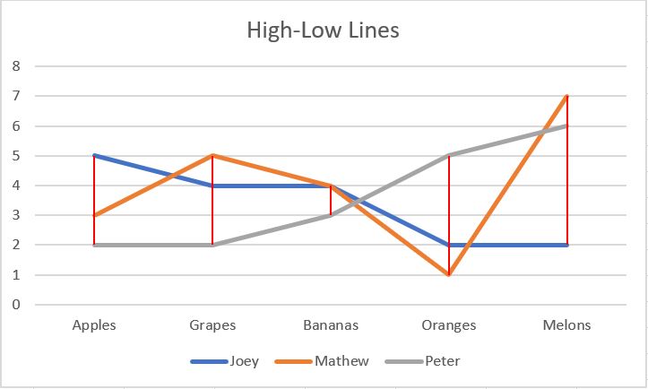
Add High-Low Lines
High-low lines are used in Excel line charts and stock charts that connect the highest and lowest points of a category.
The following code snippet shows how to add High-low lines in a stock chart.
using (ExcelEngine engine = new ExcelEngine())
{
  IApplication application = engine.Excel;
  application.DefaultVersion = ExcelVersion.Excel2013;
  FileStream fileStream = new FileStream("Sample.xlsx", FileMode.Open, FileAccess.Read);
  IWorkbook workbook = application.Workbooks.Open(fileStream);
  IWorksheet worksheet = workbook.Worksheets[0];

  IChartShape chart = worksheet.Charts[0];
  IChartSerie chartSerie = chart.Series[0];

  //Set HasHighLowLines property to true.
  chartSerie.SerieFormat.CommonSerieOptions.HasHighLowLines = true;

  //Apply formats to HighLowLines.
  chartSerie.SerieFormat.CommonSerieOptions.HighLowLines.LineColor = Color. Blue;

  FileStream stream = new FileStream("HighLowLines.xlsx", FileMode.Create,   FileAccess.ReadWrite);
  workbook.SaveAs(stream);
  stream.Dispose();
  workbook.Close();
}
using (ExcelEngine engine = new ExcelEngine())
{
IApplication application = engine.Excel;
IWorkbook workbook = application.Workbooks.Open("Sample.xlsx");
IWorksheet worksheet = workbook.Worksheets[0];
IChartShape chart = worksheet.Charts[0];
IChartSerie chartSerie = chart.Series[0];
//Set HasHighLowLines property to true.
chartSerie.SerieFormat.CommonSerieOptions.HasHighLowLines = true;
//Apply formats to HighLowLines.
chartSerie.SerieFormat.CommonSerieOptions.HighLowLines.LineColor = Color.Blue;
workbook.SaveAs("HighLowLines.xlsx");
workbook.Close();
}Using engine As ExcelEngine = New ExcelEngine()
Dim application As IApplication = engine.Excel
Dim workbook As IWorkbook = application.Workbooks.Open("Sample.xlsx")
Dim worksheet As IWorksheet = workbook.Worksheets(0)
Dim chart As IChartShape = worksheet.Charts(0)
Dim chartSerie As IChartSerie = chart.Series(0)
‘Set HasHighLowLines property to true.
chartSerie.SerieFormat.CommonSerieOptions.HasHighLowLines = True;
‘Apply formats to HighLowLines.
chartSerie.SerieFormat.CommonSerieOptions.HighLowLines.LineColor = Color.Blue
workbook.SaveAs("HighLowLines.xlsx")
workbook.Close()
End UsingA complete working example to show high low lines of chart in C# is present on this GitHub page.
The following screen shot shows the high-low lines in the line chart.
Add Drop Lines
Drop lines are used in Excel area and line charts that helps viewers to determine the data point down to the horizontal axis.
The following code snippet shows how to add Drop lines in a stock chart.
using (ExcelEngine engine = new ExcelEngine())
{
  IApplication application = engine.Excel;
  application.DefaultVersion = ExcelVersion.Excel2013;
  FileStream fileStream = new FileStream("Sample.xlsx", FileMode.Open,    FileAccess.Read);
  IWorkbook workbook = application.Workbooks.Open(fileStream);
  IWorksheet worksheet = workbook.Worksheets[0];

  IChartShape chart = worksheet.Charts[0];
  IChartSerie chartSerie = chart.Series[0];

  //Set HasDropLines property to true.
  chartSerie.SerieFormat.CommonSerieOptions.HasDropLines = true;

  //Apply formats to DropLines.
  chartSerie.SerieFormat.CommonSerieOptions.DropLines.LineColor = Color.Green;

  FileStream stream = new FileStream("DropLines.xlsx", FileMode.Create,   FileAccess.ReadWrite);
  workbook.SaveAs(stream);
  stream.Dispose();
  workbook.Close();
}
using (ExcelEngine engine = new ExcelEngine())
{
IApplication application = engine.Excel;
IWorkbook workbook = application.Workbooks.Open("Sample.xlsx");
IWorksheet worksheet = workbook.Worksheets[0];
IChartShape chart = worksheet.Charts[0];
IChartSerie chartSerie = chart.Series[0];
//Set HasDropLines property to true.
chartSerie.SerieFormat.CommonSerieOptions.HasDropLines = true;
//Apply formats to DropLines.
chartSerie.SerieFormat.CommonSerieOptions.DropLines.LineColor = Color.Green;
workbook.SaveAs("DropLines.xlsx");
workbook.Close();
}Using engine As ExcelEngine = New ExcelEngine()
Dim application As IApplication = engine.Excel
Dim workbook As IWorkbook = application.Workbooks.Open("Sample.xlsx")
Dim worksheet As IWorksheet = workbook.Worksheets(0)
Dim chart As IChartShape = worksheet.Charts(0)
Dim chartSerie As IChartSerie = chart.Series(0)
‘Set HasDropLines property to true.
chartSerie.SerieFormat.CommonSerieOptions.HasDropLines = True;
‘Apply formats to DropLines.
chartSerie.SerieFormat.CommonSerieOptions.DropLines.LineColor = Color.Green
workbook.SaveAs("DropLines.xlsx")
workbook.Close()
End UsingA complete working example to add drop lines of chart in C# is present on this GitHub page.
The following screen shot shows the drop lines in the line chart.

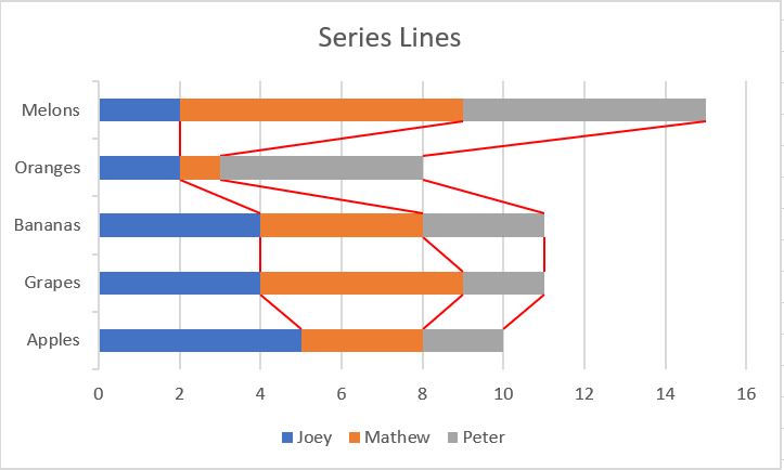
Add Series Lines
Series lines are used in Excel stacked bar and column charts that create lines from one bar to another that connect every data point in a series.
Series lines in Excel Pie-of-pie and bar-of-pie charts are used to create lines that connect the main pie chart with the secondary pie or bar chart.
The following code snippet shows how to add series lines in a pie chart.
using (ExcelEngine engine = new ExcelEngine())
{
  IApplication application = engine.Excel;
  application.DefaultVersion = ExcelVersion.Excel2013;
  FileStream fileStream = new FileStream("Sample.xlsx", FileMode.Open,    FileAccess.Read);
  IWorkbook workbook = application.Workbooks.Open(fileStream);
  IWorksheet worksheet = workbook.Worksheets[0];

  IChartShape chart = worksheet.Charts[0];
  IChartSerie chartSerie = chart.Series[0];

  //Set HasSeriesLines property to true.
  chartSerie.SerieFormat.CommonSerieOptions.HasSeriesLines = true;

  //Apply formats to SeriesLines.
  chartSerie.SerieFormat.CommonSerieOptions.PieSeriesLine.LineColor = Color.Red;

  FileStream stream = new FileStream("SeriesLines.xlsx", FileMode.Create,   FileAccess.ReadWrite);
  workbook.SaveAs(stream);
  stream.Dispose();
  workbook.Close();
}
using (ExcelEngine engine = new ExcelEngine())
{
IApplication application = engine.Excel;
IWorkbook workbook = application.Workbooks.Open("Sample.xlsx");
IWorksheet worksheet = workbook.Worksheets[0];
IChartShape chart = worksheet.Charts[0];
IChartSerie chartSerie = chart.Series[0];
//Set HasSeriesLines property to true.
chartSerie.SerieFormat.CommonSerieOptions.HasSeriesLines = true;
//Apply formats to SeriesLines.
chartSerie.SerieFormat.CommonSerieOptions.PieSeriesLine.LineColor = Color.Red;
workbook.SaveAs("SeriesLines.xlsx");
workbook.Close();
}Using engine As ExcelEngine = New ExcelEngine()
Dim application As IApplication = engine.Excel
Dim workbook As IWorkbook = application.Workbooks.Open("Sample.xlsx")
Dim worksheet As IWorksheet = workbook.Worksheets(0)
Dim chart As IChartShape = worksheet.Charts(0)
Dim chartSerie As IChartSerie = chart.Series(0)
‘Set HasSeriesLines property to true.
chartSerie.SerieFormat.CommonSerieOptions.HasSeriesLines = True;
‘Apply formats to SeriesLines.
chartSerie.SerieFormat.CommonSerieOptions.PieSeriesLine.LineColor = Color.Red
workbook.SaveAs("SeriesLines.xlsx")
workbook.Close()
End UsingA complete working example to add series lines of chart in C# is present on this GitHub page.
The following screen shot shows the series lines in the stacker bar chart.
Fill Chart Elements with Picture
Chart elements helps in modifying the chart appearance. The different chart elements are plot area, chart area, axes, titles, data points, legend, and data labels.
Fill plot area with picture
Plot area holds the data series of a chart. This plot area can be filled with solid colors, texture, picture, and pattern.
Essential XlsIO allows you to fill plot area with picture using the UserPicture of IFill interface. Refer to the following complete code snippets.
using (ExcelEngine excelEngine = new ExcelEngine())
{
  IApplication application = excelEngine.Excel;
  application.DefaultVersion = ExcelVersion.Excel2013;
  FileStream fileStream = new FileStream("Sample.xlsx", FileMode.Open, FileAccess.Read);
  IWorkbook workbook = application.Workbooks.Open(fileStream);
  IWorksheet worksheet = workbook.Worksheets[0];

  //Adding chart in the worksheet
  IChartShape chart = worksheet.Charts.Add();
  chart.DataRange = worksheet.Range["A1:C6"];
  chart.ChartType = ExcelChartType.Column_Clustered;
  chart.IsSeriesInRows = false;

  //Getting an image from the stream
  FileStream imageStream = new FileStream("Image.png", FileMode.Open, FileAccess.Read);
  Image image = Image.FromStream(imageStream);

  //Filling plot area of the chart with picture
  chart.PlotArea.Fill.UserPicture(image, "Image");

  //Saving the workbook as stream
  FileStream stream = new FileStream("Output.xlsx", FileMode.Create, FileAccess.ReadWrite);
  workbook.SaveAs(stream);
  stream.Dispose();
}
using (ExcelEngine excelEngine = new ExcelEngine())
{
IApplication application = excelEngine.Excel;
application.DefaultVersion = ExcelVersion.Excel2013;
IWorkbook workbook = application.Workbooks.Open("Sample.xlsx");
IWorksheet worksheet = workbook.Worksheets[0];
//Adding chart in the worksheet
IChartShape chart = worksheet.Charts.Add();
chart.DataRange = worksheet.Range["A1:C6"];
chart.ChartType = ExcelChartType.Column_Clustered;
chart.IsSeriesInRows = false;
//Filling plot area of the chart with picture
chart.PlotArea.Fill.UserPicture("Image.png");
workbook.SaveAs("Output.xlsx");
}Using excelEngine As ExcelEngine = New ExcelEngine()
Dim application As IApplication = excelEngine.Excel
application.DefaultVersion = ExcelVersion.Excel2013
Dim workbook As IWorkbook = application.Workbooks.Open("Sample.xlsx")
Dim worksheet As IWorksheet = workbook.Worksheets(0)
'Adding chart in the worksheet
Dim chart As IChartShape = worksheet.Charts.Add
chart.DataRange = worksheet.Range("A1:C6")
chart.ChartType = ExcelChartType.Column_Clustered
chart.IsSeriesInRows = False
'Filling plot area of the chart with picture
chart.PlotArea.Fill.UserPicture("Image.png")
workbook.SaveAs("Output.xlsx")
End UsingA complete working example to fill plot area with picture in C# is present on this GitHub page.
Fill chart area with picture
Chart area holds plot area, legend, axes, data table, and so on. This chart area can be filled with solid colors, texture, picture, and pattern.
Similar to plot area, chart area can be filled with picture using UserPicture of IFill interface. Refer to the following complete code snippets.
using (ExcelEngine excelEngine = new ExcelEngine())
{
  IApplication application = excelEngine.Excel;
  application.DefaultVersion = ExcelVersion.Excel2013;
  FileStream fileStream = new FileStream("Sample.xlsx", FileMode.Open, FileAccess.Read);
  IWorkbook workbook = application.Workbooks.Open(fileStream);
  IWorksheet worksheet = workbook.Worksheets[0];

  //Adding chart in the worksheet
  IChartShape chart = worksheet.Charts.Add();
  chart.DataRange = worksheet.Range["A1:C6"];
  chart.ChartType = ExcelChartType.Column_Clustered;
  chart.IsSeriesInRows = false;

  //Getting an image from the stream
  FileStream imageStream = new FileStream("Image.png", FileMode.Open, FileAccess.Read);
  Image image = Image.FromStream(imageStream);

  //Filling chart area of the chart with picture
  chart.ChartArea.Fill.UserPicture(image, "Image");

  //Saving the workbook as stream
  FileStream stream = new FileStream("Output.xlsx", FileMode.Create, FileAccess.ReadWrite);
  workbook.SaveAs(stream);
  stream.Dispose();
}
using (ExcelEngine excelEngine = new ExcelEngine())
{
IApplication application = excelEngine.Excel;
application.DefaultVersion = ExcelVersion.Excel2013;
IWorkbook workbook = application.Workbooks.Open("Sample.xlsx");
IWorksheet worksheet = workbook.Worksheets[0];
//Adding chart in the worksheet
IChartShape chart = worksheet.Charts.Add();
chart.DataRange = worksheet.Range["A1:C6"];
chart.ChartType = ExcelChartType.Column_Clustered;
chart.IsSeriesInRows = false;
//Filling chart area of the chart with picture
chart.ChartArea.Fill.UserPicture("Image.png");
workbook.SaveAs("Output.xlsx");
}Using excelEngine As ExcelEngine = New ExcelEngine()
Dim application As IApplication = excelEngine.Excel
application.DefaultVersion = ExcelVersion.Excel2013
Dim workbook As IWorkbook = application.Workbooks.Open("Sample.xlsx")
Dim worksheet As IWorksheet = workbook.Worksheets(0)
'Adding chart in the worksheet
Dim chart As IChartShape = worksheet.Charts.Add
chart.DataRange = worksheet.Range("A1:C6")
chart.ChartType = ExcelChartType.Column_Clustered
chart.IsSeriesInRows = False
'Filling chart area of the chart with picture
chart.ChartArea.Fill.UserPicture("Image.png")
workbook.SaveAs("Output.xlsx")
End UsingA complete working example to fill chart area with picture in C# is present on this GitHub page.
Applying 3D Formats
The following code example explains how to apply 3D settings such as rotation, side wall, back wall, and floor settings.
using (ExcelEngine excelEngine = new ExcelEngine())
{
  IApplication application = excelEngine.Excel;
  application.DefaultVersion = ExcelVersion.Excel2013;
  IWorkbook workbook = application.Workbooks.Create(2);
  IWorksheet sheet = workbook.Worksheets[0];

  //Insert the data in sheet-1
  sheet.Range["B1"].Text = "Product-A";
  sheet.Range["C1"].Text = "Product-B";
  sheet.Range["D1"].Text = "Product-C";
  sheet.Range["A2"].Text = "Jan";
  sheet.Range["A3"].Text = "Feb";
  sheet.Range["B2"].Number = 25;
  sheet.Range["B3"].Number = 20;
  sheet.Range["C2"].Number = 35;
  sheet.Range["C3"].Number = 25;
  sheet.Range["D2"].Number = 40;
  sheet.Range["D3"].Number = 55;

  IChartShape chart = sheet.Charts.Add();
  chart.DataRange = sheet.Range["A1:D3"];
  chart.ChartType = ExcelChartType.Column_Clustered_3D;

  //Set Rotation of the 3D chart view
  chart.Rotation = 90;

  //Set Back wall fill option
  chart.BackWall.Fill.FillType = ExcelFillType.Gradient;
  //Set Back wall thickness
  chart.BackWall.Thickness = 10;
  //Set Texture Type
  chart.BackWall.Fill.GradientColorType = ExcelGradientColor.TwoColor;
  chart.BackWall.Fill.GradientStyle = ExcelGradientStyle.Diagonl_Down;
  chart.BackWall.Fill.ForeColor = Color.WhiteSmoke;
  chart.BackWall.Fill.BackColor = Color.LightBlue;

  //Set side wall fill option
  chart.SideWall.Fill.FillType = ExcelFillType.SolidColor;
  //Set side wall fore and back color
  chart.SideWall.Fill.BackColor = Color.White;
  chart.SideWall.Fill.ForeColor = Color.White;

  //Set floor fill option
  chart.Floor.Fill.FillType = ExcelFillType.Pattern;
  chart.Floor.Fill.Pattern = ExcelGradientPattern.Pat_10_Percent.Pat_30_Percent;
  //Set floor fore and Back color
  chart.Floor.Fill.ForeColor = Color.Blue;
  chart.Floor.Fill.BackColor = Color.White;
  //Set floor thickness
  chart.Floor.Thickness = 3;

  //Saving the workbook as stream
  FileStream stream = new FileStream("Chart.xlsx", FileMode.Create, FileAccess.ReadWrite);
  workbook.SaveAs(stream);
  stream.Dispose();
}
using (ExcelEngine excelEngine = new ExcelEngine())
{
IApplication application = excelEngine.Excel;
application.DefaultVersion = ExcelVersion.Excel2013;
IWorkbook workbook = application.Workbooks.Create(2);
IWorksheet sheet = workbook.Worksheets[0];
//Insert the data in sheet-1
sheet.Range["B1"].Text = "Product-A";
sheet.Range["C1"].Text = "Product-B";
sheet.Range["D1"].Text = "Product-C";
sheet.Range["A2"].Text = "Jan";
sheet.Range["A3"].Text = "Feb";
sheet.Range["B2"].Number = 25;
sheet.Range["B3"].Number = 20;
sheet.Range["C2"].Number = 35;
sheet.Range["C3"].Number = 25;
sheet.Range["D2"].Number = 40;
sheet.Range["D3"].Number = 55;
IChartShape chart = sheet.Charts.Add();
chart.DataRange = sheet.Range["A1:D3"];
chart.ChartType = ExcelChartType.Column_Clustered_3D;
//Set Rotation of the 3D chart view
chart.Rotation = 90;
//Set Back wall fill option
chart.BackWall.Fill.FillType = ExcelFillType.Gradient;
//Set Back wall thickness
chart.BackWall.Thickness = 10;
//Set Texture Type
chart.BackWall.Fill.GradientColorType = ExcelGradientColor.TwoColor;
chart.BackWall.Fill.GradientStyle = ExcelGradientStyle.Diagonl_Down;
chart.BackWall.Fill.ForeColor = Color.WhiteSmoke;
chart.BackWall.Fill.BackColor = Color.LightBlue;
//Set side wall fill option
chart.SideWall.Fill.FillType = ExcelFillType.SolidColor;
//Set side wall fore and back color
chart.SideWall.Fill.BackColor = Color.White;
chart.SideWall.Fill.ForeColor = Color.White;
//Set floor fill option
chart.Floor.Fill.FillType = ExcelFillType.Pattern;
chart.Floor.Fill.Pattern = ExcelGradientPattern.Pat_10_Percent.Pat_30_Percent;
//Set floor fore and Back color
chart.Floor.Fill.ForeColor = Color.Blue;
chart.Floor.Fill.BackColor = Color.White;
//Set floor thickness
chart.Floor.Thickness = 3;
workbook.SaveAs("Chart.xlsx");
}Using excelEngine As ExcelEngine = New ExcelEngine()
Dim application As IApplication = excelEngine.Excel
application.DefaultVersion = ExcelVersion.Excel2013
Dim workbook As IWorkbook = application.Workbooks.Create(2)
Dim sheet As IWorksheet = workbook.Worksheets(0)
'Insert data in sheet-1
sheet.Range("B1").Text = "Product-A"
sheet.Range("C1").Text = "Product-B"
sheet.Range("D1").Text = "Product-C"
sheet.Range("A2").Text = "Jan"
sheet.Range("A3").Text = "Feb"
sheet.Range("B2").Number = 25
sheet.Range("B3").Number = 20
sheet.Range("C2").Number = 35
sheet.Range("C3").Number = 25
sheet.Range("D2").Number = 40
sheet.Range("D3").Number = 55
Dim chart As IChartShape = sheet.Charts.Add()
chart.DataRange = sheet.Range("A1:D3")
chart.ChartType = ExcelChartType.Column_Clustered_3D
'Set Rotation of the 3D chart view
chart.Rotation = 90
'Set Back wall fill option
chart.BackWall.Fill.FillType = ExcelFillType.Gradient
'Set Texture Type
chart.BackWall.Fill.GradientColorType = ExcelGradientColor.TwoColor
chart.BackWall.Fill.GradientStyle = ExcelGradientStyle.Diagonl_Down
chart.BackWall.Fill.ForeColor = Color.WhiteSmoke
chart.BackWall.Fill.BackColor = Color.LightBlue
'Set Back wall thickness
chart.BackWall.Thickness = 10
'Set side wall fill option
chart.SideWall.Fill.FillType = ExcelFillType.SolidColor
'Set sidewall fore and back color
chart.SideWall.Fill.BackColor = Color.White
chart.SideWall.Fill.ForeColor = Color.White
'Set floor fill option
chart.Floor.Fill.FillType = ExcelFillType.Pattern
chart.Floor.Fill.Pattern = ExcelGradientPattern.Pat_10_Percent.Pat_30_Percent
'Set floor fore and Back color
chart.Floor.Fill.ForeColor = Color.Blue
chart.Floor.Fill.BackColor = Color.White
'Set floor thickness
chart.Floor.Thickness = 3
workbook.SaveAs("Chart.xlsx")
End UsingA complete working example for 3D chart formats in C# is present on this GitHub page.
Customizing chart and Chart Elements
Positioning Chart
Chart can be positioned by specifying row and column indexes. The following code samples illustrates how to position a chart in a worksheet.
//Positioning chart in a worksheet
chart.TopRow = 5;
chart.LeftColumn = 5;
chart.RightColumn = 10;
chart.BottomRow = 10;
//Positioning chart in a worksheet
chart.TopRow = 5;
chart.LeftColumn = 5;
chart.RightColumn = 10;
chart.BottomRow = 10;'Positioning chart in a worksheet
chart.TopRow = 5
chart.LeftColumn = 5
chart.RightColumn = 10
chart.BottomRow = 10Positioning Chart Elements
The following code examples illustrate how to position the chart elements.
//Manually positioning chart plot area using Layout
chart.PlotArea.Layout.LayoutTarget = LayoutTargets.inner;
chart.PlotArea.Layout.LeftMode = LayoutModes.edge;
chart.PlotArea.Layout.TopMode = LayoutModes.edge;
//Manually positioning chart plot area using Manual Layout
chart.PlotArea.Layout.ManualLayout.LayoutTarget = LayoutTargets.inner;
chart.PlotArea.Layout.ManualLayout.LeftMode = LayoutModes.edge;
chart.PlotArea.Layout.ManualLayout.TopMode = LayoutModes.edge;
//Manually positioning chart legend area using Layout
chart.Legend.Layout.LeftMode = LayoutModes.edge;
chart.Legend.Layout.TopMode = LayoutModes.edge;
//Manually positioning chart legend area using Manual Layout
chart.Legend.Layout.ManualLayout.LeftMode = LayoutModes.edge;
chart.Legend.Layout.ManualLayout.TopMode = LayoutModes.edge;//Manually positioning chart plot area using Layout
chart.PlotArea.Layout.LayoutTarget = LayoutTargets.inner;
chart.PlotArea.Layout.LeftMode = LayoutModes.edge;
chart.PlotArea.Layout.TopMode = LayoutModes.edge;
//Manually positioning chart plot area using Manual Layout
chart.PlotArea.Layout.ManualLayout.LayoutTarget = LayoutTargets.inner;
chart.PlotArea.Layout.ManualLayout.LeftMode = LayoutModes.edge;
chart.PlotArea.Layout.ManualLayout.TopMode = LayoutModes.edge;
//Manually positioning chart legend area using Layout
chart.Legend.Layout.LeftMode = LayoutModes.edge;
chart.Legend.Layout.TopMode = LayoutModes.edge;
//Manually positioning chart legend area using Manual Layout
chart.Legend.Layout.ManualLayout.LeftMode = LayoutModes.edge;
chart.Legend.Layout.ManualLayout.TopMode = LayoutModes.edge;'Manually positioning chart plot area using Layout
chart.PlotArea.Layout.LayoutTarget = LayoutTargets.inner
chart.PlotArea.Layout.LeftMode = LayoutModes.edge
chart.PlotArea.Layout.TopMode = LayoutModes.edge
'Manually positioning chart plot area using Manual Layout
chart.PlotArea.Layout.ManualLayout.LayoutTarget = LayoutTargets.inner;
chart.PlotArea.Layout.ManualLayout.LeftMode = LayoutModes.edge;
chart.PlotArea.Layout.ManualLayout.TopMode = LayoutModes.edge;
'Manually positioning chart legend area using Layout
chart.Legend.Layout.LeftMode = LayoutModes.edge
chart.Legend.Layout.TopMode = LayoutModes.edge
'Manually positioning chart legend area using Manual Layout
chart.Legend.Layout.ManualLayout.LeftMode = LayoutModes.edge;
chart.Legend.Layout.ManualLayout.TopMode = LayoutModes.edge;Resizing Chart
The following code sample illustrates how to resize a chart in a worksheet.
IShape chartShape = chart as IShape;
//Set Height of the chart in pixels
chartShape.Height = 300;
//Set Width of the chart
chartShape.Width = 500;IShape chartShape = chart as IShape;
//Set Height of the chart in pixels
chartShape.Height = 300;
//Set Width of the chart
chartShape.Width = 500;Dim chartShape As IShape = chart as IShape
'Set Height of the chart
chartShape.Height = 300
'Set Width of the chart
chartShape.Width = 500Resizing Chart Elements
The following code examples illustrate how to resize chart elements such as plot area and legend.
//Manually resizing chart plot area using Layout
chart.PlotArea.Layout.Left = 70;
chart.PlotArea.Layout.Top = 40;
chart.PlotArea.Layout.Width = 280;
chart.PlotArea.Layout.Height = 200;
//Manually resizing chart plot area using Manual Layout
chart.PlotArea.Layout.ManualLayout.Height = 0.80;
chart.PlotArea.Layout.ManualLayout.Width = 0.65;
chart.PlotArea.Layout.ManualLayout.Top = 0.03;
chart.PlotArea.Layout.ManualLayout.Left = -0.1;
//Manually resizing chart legend area using Layout
chart.Legend.Layout.Left = 400;
chart.Legend.Layout.Top = 150;
chart.Legend.Layout.Width = 150;
chart.Legend.Layout.Height = 100;
//Manually resizing chart legend area using Manual Layout
chart.Legend.Layout.ManualLayout.Height = 0.09;
chart.Legend.Layout.ManualLayout.Width = 0.30;
chart.Legend.Layout.ManualLayout.Top = 0.36;
chart.Legend.Layout.ManualLayout.Left = 0.68;
//Manually resizing chart title area using Layout
chart.ChartTitleArea.Text = "Sample Chart";
chart.ChartTitleArea.Layout.Top = 10;
chart.ChartTitleArea.Layout.Left = 150;
//Manually resizing chart title area using Manual Layout
chart.ChartTitleArea.Text = "Sample Chart";
chart.ChartTitleArea.Layout.ManualLayout.Top = 0.005;
chart.ChartTitleArea.Layout.ManualLayout.Left = 0.26;
//Manually resizing axis title area using Layout
chart.PrimaryValueAxis.TitleArea.Layout.Left = 15;
chart.PrimaryValueAxis.TitleArea.Layout.Top = 20;
chart.PrimaryCategoryAxis.TitleArea.Layout.Left = 25;
chart.PrimaryCategoryAxis.TitleArea.Layout.Top = 20;
//Manually resizing axis title area using Manual Layout
chart.PrimaryValueAxis.TitleArea.Layout.ManualLayout.Left = 0.04;
chart.PrimaryValueAxis.TitleArea.Layout.ManualLayout.Top = 0.34;
chart.PrimaryCategoryAxis.TitleArea.Layout.ManualLayout.Left = 0.38;
chart.PrimaryCategoryAxis.TitleArea.Layout.ManualLayout.Top = 0.95;
//Manually resizing data label area using Layout
chart.Series[0].DataPoints[0].DataLabels.Layout.Left = 0.09;
chart.Series[0].DataPoints[0].DataLabels.Layout.Top = 0.01;
//Manually resizing data label area using Manual Layout
chart.Series[0].DataPoints[0].DataLabels.Layout.ManualLayout.Left = 0.09;
chart.Series[0].DataPoints[0].DataLabels.Layout.ManualLayout.Top = 0.01;//Manually resizing chart plot area using Layout
chart.PlotArea.Layout.Left = 70;
chart.PlotArea.Layout.Top = 40;
chart.PlotArea.Layout.Width = 280;
chart.PlotArea.Layout.Height = 200;
//Manually resizing chart plot area using Manual Layout
chart.PlotArea.Layout.ManualLayout.Height = 0.80;
chart.PlotArea.Layout.ManualLayout.Width = 0.65;
chart.PlotArea.Layout.ManualLayout.Top = 0.03;
chart.PlotArea.Layout.ManualLayout.Left = -0.1;
//Manually resizing chart legend area using Layout
chart.Legend.Layout.Left = 400;
chart.Legend.Layout.Top = 150;
chart.Legend.Layout.Width = 150;
chart.Legend.Layout.Height = 100;
//Manually resizing chart legend area using Manual Layout
chart.Legend.Layout.ManualLayout.Height = 0.09;
chart.Legend.Layout.ManualLayout.Width = 0.30;
chart.Legend.Layout.ManualLayout.Top = 0.36;
chart.Legend.Layout.ManualLayout.Left = 0.68;
//Manually resizing chart title area using Layout
chart.ChartTitleArea.Text = "Sample Chart";
chart.ChartTitleArea.Layout.Top = 10;
chart.ChartTitleArea.Layout.Left = 150;
//Manually resizing chart title area using Manual Layout
chart.ChartTitleArea.Text = "Sample Chart";
chart.ChartTitleArea.Layout.ManualLayout.Top = 0.005;
chart.ChartTitleArea.Layout.ManualLayout.Left = 0.26;
//Manually resizing axis title area using Layout
chart.PrimaryValueAxis.TitleArea.Layout.Left = 15;
chart.PrimaryValueAxis.TitleArea.Layout.Top = 20;
chart.PrimaryCategoryAxis.TitleArea.Layout.Left = 25;
chart.PrimaryCategoryAxis.TitleArea.Layout.Top = 20;
//Manually resizing axis title area using Manual Layout
chart.PrimaryValueAxis.TitleArea.Layout.ManualLayout.Left = 0.04;
chart.PrimaryValueAxis.TitleArea.Layout.ManualLayout.Top = 0.34;
chart.PrimaryCategoryAxis.TitleArea.Layout.ManualLayout.Left = 0.38;
chart.PrimaryCategoryAxis.TitleArea.Layout.ManualLayout.Top = 0.95;
//Manually resizing data label area using Layout
chart.Series[0].DataPoints[0].DataLabels.Layout.Left = 0.09;
chart.Series[0].DataPoints[0].DataLabels.Layout.Top = 0.01;
//Manually resizing data label area using Manual Layout
chart.Series[0].DataPoints[0].DataLabels.Layout.ManualLayout.Left = 0.09;
chart.Series[0].DataPoints[0].DataLabels.Layout.ManualLayout.Top = 0.01;'Manually resizing chart plot area using Layout
chart.PlotArea.Layout.Left = 70
chart.PlotArea.Layout.Top = 40
chart.PlotArea.Layout.Width = 280
chart.PlotArea.Layout.Height = 200
'Manually resizing chart plot area using Manual Layout
chart.PlotArea.Layout.ManualLayout.Height = 0.80
chart.PlotArea.Layout.ManualLayout.Width = 0.65
chart.PlotArea.Layout.ManualLayout.Top = 0.03
chart.PlotArea.Layout.ManualLayout.Left = -0.1
'Manually resizing chart legend area using Layout
chart.Legend.Layout.Left = 400
chart.Legend.Layout.Top = 150
chart.Legend.Layout.Width = 150
chart.Legend.Layout.Height = 100
'Manually resizing chart legend area using Manual Layout
chart.Legend.Layout.ManualLayout.Height = 0.09
chart.Legend.Layout.ManualLayout.Width = 0.30
chart.Legend.Layout.ManualLayout.Top = 0.36
chart.Legend.Layout.ManualLayout.Left = 0.68
'Manually resizing chart title area using Layout
chart.ChartTitleArea.Text = "Sample Chart"
chart.ChartTitleArea.Layout.Top = 10
chart.ChartTitleArea.Layout.Left = 150
'Manually resizing chart title area using Manual Layout
chart.ChartTitleArea.Text = "Sample Chart"
chart.ChartTitleArea.Layout.ManualLayout.Top = 0.005
chart.ChartTitleArea.Layout.ManualLayout.Left = 0.26
'Manually resizing axis title area using Layout
chart.PrimaryValueAxis.TitleArea.Layout.Left = 15
chart.PrimaryValueAxis.TitleArea.Layout.Top = 20
chart.PrimaryCategoryAxis.TitleArea.Layout.Left = 25
chart.PrimaryCategoryAxis.TitleArea.Layout.Top = 20
'Manually resizing axis title area using Manual Layout
chart.PrimaryValueAxis.TitleArea.Layout.ManualLayout.Left = 0.04
chart.PrimaryValueAxis.TitleArea.Layout.ManualLayout.Top = 0.34
chart.PrimaryCategoryAxis.TitleArea.Layout.ManualLayout.Left = 0.38
chart.PrimaryCategoryAxis.TitleArea.Layout.ManualLayout.Top = 0.95
'Manually resizing data label area using Layout
chart.Series(0).DataPoints(0).DataLabels.Layout.Left = 0.09
chart.Series(0).DataPoints(0).DataLabels.Layout.Top = 0.01
'Manually resizing data label area using Manual Layout
chart.Series(0).DataPoints(0).DataLabels.Layout.ManualLayout.Left = 0.09
chart.Series(0).DataPoints(0).DataLabels.Layout.ManualLayout.Top = 0.01Chart with transparent background
The following code example explains how to apply transparency to chart area.
//Applying transparency to chart area
chart.ChartArea.Fill.Transparency = 0.5;//Applying transparency to chart area
chart.ChartArea.Fill.Transparency = 0.5;'Applying transparency to chart area
chart.ChartArea.Fill.Transparency = 0.5The complete code snippet illustrating the above options is shown below.
using (ExcelEngine excelEngine = new ExcelEngine())
{
IApplication application = excelEngine.Excel;
application.DefaultVersion = ExcelVersion.Xlsx;
FileStream inputStream = new FileStream("Sample.xlsx", FileMode.Open, FileAccess.Read);
IWorkbook workbook = application.Workbooks.Open(inputStream);
//Positioning chart elements using layout
//Access the first sheet in the workbook
IWorksheet sheet = workbook.Worksheets[0];
IChartShape chart = sheet.Charts[0];
//Positioning chart in a worksheet
chart.TopRow = 5;
chart.LeftColumn = 5;
chart.RightColumn = 10;
chart.BottomRow = 10;
//Manually positioning chart plot area
chart.PlotArea.Layout.LayoutTarget = LayoutTargets.inner;
chart.PlotArea.Layout.LeftMode = LayoutModes.edge;
chart.PlotArea.Layout.TopMode = LayoutModes.edge;
//Manually positioning chart legend area
chart.Legend.Layout.LeftMode = LayoutModes.edge;
chart.Legend.Layout.TopMode = LayoutModes.edge;
IShape chartShape = chart as IShape;
//Set Height of the chart in pixels
chartShape.Height = 300;
//Set Width of the chart
chartShape.Width = 500;
//Manually resizing chart plot area
chart.PlotArea.Layout.Left = 70;
chart.PlotArea.Layout.Top = 40;
chart.PlotArea.Layout.Width = 280;
chart.PlotArea.Layout.Height = 200;
//Manually resizing chart legend area
chart.Legend.Layout.Left = 400;
chart.Legend.Layout.Top = 150;
chart.Legend.Layout.Width = 150;
chart.Legend.Layout.Height = 100;
// Manually resizing chart title area
chart.ChartTitleArea.Text = "Sample Chart";
chart.ChartTitleArea.Layout.Top = 10;
chart.ChartTitleArea.Layout.Left = 150;
// Manually resizing axis title area
chart.PrimaryValueAxis.TitleArea.Layout.Left = 15;
chart.PrimaryValueAxis.TitleArea.Layout.Top = 20;
chart.PrimaryCategoryAxis.TitleArea.Layout.Left = 25;
chart.PrimaryCategoryAxis.TitleArea.Layout.Top = 20;
// Manually resizing data label area
chart.Series[0].DataPoints[0].DataLabels.Layout.Left = 0.09;
chart.Series[0].DataPoints[0].DataLabels.Layout.Top = 0.01;
//Applying transparency to chart area
chart.ChartArea.Fill.Transparency = 0.5;
//Positioning chart elements using manual layout
//Access the second sheet in the workbook
IWorksheet sheet1 = workbook.Worksheets[1];
IChartShape chart1 = sheet1.Charts[0];
//Positioning chart in a worksheet
chart1.TopRow = 5;
chart1.LeftColumn = 5;
chart1.RightColumn = 10;
chart1.BottomRow = 10;
//Manually positioning chart plot area
chart1.PlotArea.Layout.ManualLayout.LayoutTarget = LayoutTargets.inner;
chart1.PlotArea.Layout.ManualLayout.LeftMode = LayoutModes.edge;
chart1.PlotArea.Layout.ManualLayout.TopMode = LayoutModes.edge;
//Manually positioning chart legend area
chart1.Legend.Layout.ManualLayout.LeftMode = LayoutModes.edge;
chart1.Legend.Layout.ManualLayout.TopMode = LayoutModes.edge;
IShape chartShape1 = chart1 as IShape;
//Set Height of the chart in pixels
chartShape1.Height = 300;
//Set Width of the chart
chartShape1.Width = 500;
//Manually resizing chart plot area
chart1.PlotArea.Layout.ManualLayout.Height = 0.80;
chart1.PlotArea.Layout.ManualLayout.Width = 0.65;
chart1.PlotArea.Layout.ManualLayout.Top = 0.03;
chart1.PlotArea.Layout.ManualLayout.Left = -0.1;
//Manually resizing chart legend area
chart1.Legend.Layout.ManualLayout.Height = 0.09;
chart1.Legend.Layout.ManualLayout.Width = 0.30;
chart1.Legend.Layout.ManualLayout.Top = 0.36;
chart1.Legend.Layout.ManualLayout.Left = 0.68;
//Manually resizing chart title area
chart1.ChartTitleArea.Text = "Sample Chart";
chart1.ChartTitleArea.Layout.ManualLayout.Top = 0.005;
chart1.ChartTitleArea.Layout.ManualLayout.Left = 0.26;
//Manually resizing axis title area
chart1.PrimaryValueAxis.TitleArea.Layout.ManualLayout.Left = 0.04;
chart1.PrimaryValueAxis.TitleArea.Layout.ManualLayout.Top = 0.34;
chart1.PrimaryCategoryAxis.TitleArea.Layout.ManualLayout.Left = 0.38;
chart1.PrimaryCategoryAxis.TitleArea.Layout.ManualLayout.Top = 0.95;
//Manually resizing data label area
chart1.Series[0].DataPoints[0].DataLabels.Layout.ManualLayout.Left = 0.09;
chart1.Series[0].DataPoints[0].DataLabels.Layout.ManualLayout.Top = 0.01;
//Applying transparency to chart area
chart1.ChartArea.Fill.Transparency = 0.5;
//Saving the workbook as stream
FileStream stream = new FileStream("Chart.xlsx", FileMode.Create, FileAccess.ReadWrite);
workbook.SaveAs(stream);
stream.Dispose();
}using (ExcelEngine excelEngine = new ExcelEngine())
{
IApplication application = excelEngine.Excel;
application.DefaultVersion = ExcelVersion.Xlsx;
IWorkbook workbook = application.Workbooks.Open("Sample.xlsx", ExcelOpenType.Automatic);
//Positioning chart elements using layout
//Access the first sheet in the workbook
IWorksheet sheet = workbook.Worksheets[0];
IChartShape chart = sheet.Charts[0];
//Positioning chart in a worksheet
chart.TopRow = 5;
chart.LeftColumn = 5;
chart.RightColumn = 10;
chart.BottomRow = 10;
//Manually positioning chart plot area
chart.PlotArea.Layout.LayoutTarget = LayoutTargets.inner;
chart.PlotArea.Layout.LeftMode = LayoutModes.edge;
chart.PlotArea.Layout.TopMode = LayoutModes.edge;
//Manually positioning chart legend area
chart.Legend.Layout.LeftMode = LayoutModes.edge;
chart.Legend.Layout.TopMode = LayoutModes.edge;
IShape chartShape = chart as IShape;
//Set Height of the chart in pixels
chartShape.Height = 300;
//Set Width of the chart
chartShape.Width = 500;
//Manually resizing chart plot area
chart.PlotArea.Layout.Left = 70;
chart.PlotArea.Layout.Top = 40;
chart.PlotArea.Layout.Width = 280;
chart.PlotArea.Layout.Height = 200;
//Manually resizing chart legend area
chart.Legend.Layout.Left = 400;
chart.Legend.Layout.Top = 150;
chart.Legend.Layout.Width = 150;
chart.Legend.Layout.Height = 100;
// Manually resizing chart title area
chart.ChartTitleArea.Text = "Sample Chart";
chart.ChartTitleArea.Layout.Top = 10;
chart.ChartTitleArea.Layout.Left = 150;
// Manually resizing axis title area
chart.PrimaryValueAxis.TitleArea.Layout.Left = 15;
chart.PrimaryValueAxis.TitleArea.Layout.Top = 20;
chart.PrimaryCategoryAxis.TitleArea.Layout.Left = 25;
chart.PrimaryCategoryAxis.TitleArea.Layout.Top = 20;
// Manually resizing data label area
chart.Series[0].DataPoints[0].DataLabels.Layout.Left = 0.09;
chart.Series[0].DataPoints[0].DataLabels.Layout.Top = 0.01;
//Applying transparency to chart area
chart.ChartArea.Fill.Transparency = 0.5;
//Positioning chart elements using manual layout
//Access the second sheet in the workbook
IWorksheet sheet1 = workbook.Worksheets[1];
IChartShape chart1 = sheet1.Charts[0];
//Positioning chart in a worksheet
chart1.TopRow = 5;
chart1.LeftColumn = 5;
chart1.RightColumn = 10;
chart1.BottomRow = 10;
//Manually positioning chart plot area
chart1.PlotArea.Layout.ManualLayout.LayoutTarget = LayoutTargets.inner;
chart1.PlotArea.Layout.ManualLayout.LeftMode = LayoutModes.edge;
chart1.PlotArea.Layout.ManualLayout.TopMode = LayoutModes.edge;
//Manually positioning chart legend area
chart1.Legend.Layout.ManualLayout.LeftMode = LayoutModes.edge;
chart1.Legend.Layout.ManualLayout.TopMode = LayoutModes.edge;
IShape chartShape1 = chart1 as IShape;
//Set Height of the chart in pixels
chartShape1.Height = 300;
//Set Width of the chart
chartShape1.Width = 500;
//Manually resizing chart plot area
chart1.PlotArea.Layout.ManualLayout.Height = 0.80;
chart1.PlotArea.Layout.ManualLayout.Width = 0.65;
chart1.PlotArea.Layout.ManualLayout.Top = 0.03;
chart1.PlotArea.Layout.ManualLayout.Left = -0.1;
//Manually resizing chart legend area
chart1.Legend.Layout.ManualLayout.Height = 0.09;
chart1.Legend.Layout.ManualLayout.Width = 0.30;
chart1.Legend.Layout.ManualLayout.Top = 0.36;
chart1.Legend.Layout.ManualLayout.Left = 0.68;
//Manually resizing chart title area
chart1.ChartTitleArea.Text = "Sample Chart";
chart1.ChartTitleArea.Layout.ManualLayout.Top = 0.005;
chart1.ChartTitleArea.Layout.ManualLayout.Left = 0.26;
//Manually resizing axis title area
chart1.PrimaryValueAxis.TitleArea.Layout.ManualLayout.Left = 0.04;
chart1.PrimaryValueAxis.TitleArea.Layout.ManualLayout.Top = 0.34;
chart1.PrimaryCategoryAxis.TitleArea.Layout.ManualLayout.Left = 0.38;
chart1.PrimaryCategoryAxis.TitleArea.Layout.ManualLayout.Top = 0.95;
//Manually resizing data label area
chart1.Series[0].DataPoints[0].DataLabels.Layout.ManualLayout.Left = 0.09;
chart1.Series[0].DataPoints[0].DataLabels.Layout.ManualLayout.Top = 0.01;
//Applying transparency to chart area
chart1.ChartArea.Fill.Transparency = 0.5;
workbook.SaveAs("Chart.xlsx");
}Using excelEngine As ExcelEngine = New ExcelEngine()
Dim application As IApplication = excelEngine.Excel
application.DefaultVersion = ExcelVersion.Xlsx
Dim workbook As IWorkbook = application.Workbooks.Open("Sample.xlsx", ExcelOpenType.Automatic)
'Positioning chart elements using layout
'Access the first sheet in the workbook
Dim sheet As IWorksheet = workbook.Worksheets(0)
Dim chart As IChartShape = sheet.Charts(0)
'Positioning chart in a worksheet
chart.TopRow = 5
chart.LeftColumn = 5
chart.RightColumn = 10
chart.BottomRow = 10
'Manually positioning chart plot area
chart.PlotArea.Layout.LayoutTarget = LayoutTargets.inner
chart.PlotArea.Layout.LeftMode = LayoutModes.edge
chart.PlotArea.Layout.TopMode = LayoutModes.edge
'Manually positioning chart legend area
chart.Legend.Layout.LeftMode = LayoutModes.edge
chart.Legend.Layout.TopMode = LayoutModes.edge
Dim chartShape As IShape = TryCast(chart, IShape)
'Set Height of the chart in pixels
chartShape.Height = 300
'Set Width of the chart
chartShape.Width = 500
'Manually resizing chart plot area
chart.PlotArea.Layout.Left = 70
chart.PlotArea.Layout.Top = 40
chart.PlotArea.Layout.Width = 280
chart.PlotArea.Layout.Height = 200
'Manually resizing chart legend area
chart.Legend.Layout.Left = 400
chart.Legend.Layout.Top = 150
chart.Legend.Layout.Width = 150
chart.Legend.Layout.Height = 100
'Manually resizing chart title area
chart.ChartTitleArea.Text = "Sample Chart"
chart.ChartTitleArea.Layout.Top = 10
chart.ChartTitleArea.Layout.Left = 150
'Manually resizing axis title area
chart.PrimaryValueAxis.TitleArea.Layout.Left = 15
chart.PrimaryValueAxis.TitleArea.Layout.Top = 20
chart.PrimaryCategoryAxis.TitleArea.Layout.Left = 25
chart.PrimaryCategoryAxis.TitleArea.Layout.Top = 20
'Manually resizing data label area
chart.Series(0).DataPoints(0).DataLabels.Layout.Left = 0.09
chart.Series(0).DataPoints(0).DataLabels.Layout.Top = 0.01
'Applying transparency to chart area
chart.ChartArea.Fill.Transparency = 0.5
'Positioning chart elements using manual layout
'Access the second sheet in the workbook
Dim sheet1 As IWorksheet = workbook.Worksheets(0)
Dim chart1 As IChartShape = sheet.Charts(0)
//Positioning chart in a worksheet
chart1.TopRow = 5
chart1.LeftColumn = 5
chart1.RightColumn = 10
chart1.BottomRow = 10
//Manually positioning chart plot area
chart1.PlotArea.Layout.ManualLayout.LayoutTarget = LayoutTargets.inner
chart1.PlotArea.Layout.ManualLayout.LeftMode = LayoutModes.edge
chart1.PlotArea.Layout.ManualLayout.TopMode = LayoutModes.edge
//Manually positioning chart legend area
chart1.Legend.Layout.ManualLayout.LeftMode = LayoutModes.edge
chart1.Legend.Layout.ManualLayout.TopMode = LayoutModes.edge
Dim chartShape1 As IShape = TryCast(chart1, IShape)
//Set Height of the chart in pixels
chartShape1.Height = 300
//Set Width of the chart
chartShape1.Width = 500
//Manually resizing chart plot area
chart1.PlotArea.Layout.ManualLayout.Height = 0.80
chart1.PlotArea.Layout.ManualLayout.Width = 0.65
chart1.PlotArea.Layout.ManualLayout.Top = 0.03
chart1.PlotArea.Layout.ManualLayout.Left = -0.1
//Manually resizing chart legend area
chart1.Legend.Layout.ManualLayout.Height = 0.09
chart1.Legend.Layout.ManualLayout.Width = 0.30
chart1.Legend.Layout.ManualLayout.Top = 0.36
chart1.Legend.Layout.ManualLayout.Left = 0.68
'Manually resizing chart title area
chart1.ChartTitleArea.Text = "Sample Chart"
chart1.ChartTitleArea.Layout.ManualLayout.Top = 0.005
chart1.ChartTitleArea.Layout.ManualLayout.Left = 0.26
'Manually resizing axis title area
chart1.PrimaryValueAxis.TitleArea.Layout.ManualLayout.Left = 0.04
chart1.PrimaryValueAxis.TitleArea.Layout.ManualLayout.Top = 0.34
chart1.PrimaryCategoryAxis.TitleArea.Layout.ManualLayout.Left = 0.38
chart1.PrimaryCategoryAxis.TitleArea.Layout.ManualLayout.Top = 0.95
'Manually resizing data label area
chart1.Series(0).DataPoints(0).DataLabels.Layout.ManualLayout.Left = 0.09
chart1.Series(0).DataPoints(0).DataLabels.Layout.ManualLayout.Top = 0.01
'Applying transparency to chart area
chart1.ChartArea.Fill.Transparency = 0.5
workbook.SaveAs("Chart.xlsx")
End UsingA complete working example explaining different chart elements in C# is present on this GitHub page.
NOTE
In order to position the chart elements, plot area should be smaller than chart area.
Explode a Pie Chart
Essential XlsIO allows you to explode either all data points at a single explosion value or each data point at different explosion using Percent of IChartSerieDataFormat interface.
You can either create a pie chart and then explode it or directly create an exploded pie chart using XlsIO. Selecting Pie_Exploded as ChartType inserts a pie chart with a default explosion of 25%. Learn how to Create an Exploded Pie Chart.
Refer the following complete code snippets.
using (ExcelEngine excelEngine = new ExcelEngine())
{
  IApplication application = excelEngine.Excel;
  application.DefaultVersion = ExcelVersion.Excel2013;
  FileStream fileStream = new FileStream("Sample.xlsx", FileMode.Open, FileAccess.Read);
  IWorkbook workbook = application.Workbooks.Open(fileStream);
  IWorksheet worksheet = workbook.Worksheets[0];

  //Adding pie chart in the worksheet
  IChartShape chart = worksheet.Charts.Add();
  chart.DataRange = worksheet.Range["A3:B7"];
  chart.ChartType = ExcelChartType.Pie;
  chart.IsSeriesInRows = false;

  //Showing the values of data points
  chart.Series[0].DataPoints.DefaultDataPoint.DataLabels.IsValue = true;

  //Exploding the pie chart to 40%
  chart.Series[0].SerieFormat.Percent = 40;

  //Saving the workbook as stream
  FileStream stream = new FileStream("Output.xlsx", FileMode.Create, FileAccess.ReadWrite);
  workbook.SaveAs(stream);
  stream.Dispose();
}
using (ExcelEngine excelEngine = new ExcelEngine())
{
IApplication application = excelEngine.Excel;
application.DefaultVersion = ExcelVersion.Excel2013;
IWorkbook workbook = application.Workbooks.Open("Sample.xlsx");
IWorksheet worksheet = workbook.Worksheets[0];
//Adding pie chart in the worksheet
IChartShape chart = worksheet.Charts.Add();
chart.DataRange = worksheet.Range["A3:B7"];
chart.ChartType = ExcelChartType.Pie;
chart.IsSeriesInRows = false;
//Showing the values of data points
chart.Series[0].DataPoints.DefaultDataPoint.DataLabels.IsValue = true;
//Exploding the pie chart to 40%
chart.Series[0].SerieFormat.Percent = 40;
workbook.SaveAs("Output.xlsx");
}Using excelEngine As ExcelEngine = New ExcelEngine()
Dim application As IApplication = excelEngine.Excel
application.DefaultVersion = ExcelVersion.Excel2013
Dim workbook As IWorkbook = application.Workbooks.Open("Sample.xlsx")
Dim worksheet As IWorksheet = workbook.Worksheets(0)
'Adding pie chart in the worksheet
Dim chart As IChartShape = worksheet.Charts.Add
chart.DataRange = worksheet.Range("A3:B7")
chart.ChartType = ExcelChartType.Pie
chart.IsSeriesInRows = False
'Showing the values of data points
chart.Series(0).DataPoints.DefaultDataPoint.DataLabels.IsValue = True
'Exploding the pie chart to 40%
chart.Series(0).SerieFormat.Percent = 40
workbook.SaveAs("Output.xlsx")
End UsingA complete working example to explode a pie chart in C# is present on this GitHub page.
Add Picture to Chart and assign Hyperlink
Essential XlsIO supports assigning hyperlink to the picture added in a chart in the Excel workbook. To achieve this, create a chart in workbook and add picture to the chart using AddPicture of IPictures interface. You can assign hyperlink to the picture using Add property of IHyperLinks interface.
Refer to the following complete code snippets.
using (ExcelEngine excelEngine = new ExcelEngine())
{
  IApplication application = excelEngine.Excel;
  application.DefaultVersion = ExcelVersion.Excel2013;
  FileStream fileStream = new FileStream("Sample.xlsx", FileMode.Open, FileAccess.Read);
  IWorkbook workbook = application.Workbooks.Open(fileStream);
  IWorksheet worksheet = workbook.Worksheets[0];

  //Adding chart in the workbook
  IChart chart = workbook.Charts.Add();
  chart.DataRange = worksheet.Range["A1:B6"];
  chart.ChartType = ExcelChartType.Column_Clustered;
  chart.IsSeriesInRows = false;

  //Getting an image from the stream
  FileStream imageStream = new FileStream("Image.png", FileMode.Open, FileAccess.Read);
  Image image = Image.FromStream(imageStream);

  //Adding picture on the chart
  chart.Pictures.AddPicture(1, 1, imageStream);

  //Adding hyperlink to the picture on chart
  worksheet.HyperLinks.Add((workbook.Charts[0].Pictures[0] as IShape), ExcelHyperLinkType.Url, "http://www.Syncfusion.com", "click here");

  //Saving the workbook as stream
  FileStream stream = new FileStream("Output.xlsx", FileMode.Create, FileAccess.ReadWrite);
  workbook.SaveAs(stream);
  stream.Dispose();
}
using (ExcelEngine excelEngine = new ExcelEngine())
{
IApplication application = excelEngine.Excel;
application.DefaultVersion = ExcelVersion.Excel2013;
IWorkbook workbook = application.Workbooks.Open("Sample.xlsx");
IWorksheet worksheet = workbook.Worksheets[0];
//Adding chart in the workbook
IChart chart = workbook.Charts.Add();
chart.DataRange = worksheet.Range["A1:B6"];
chart.ChartType = ExcelChartType.Column_Clustered;
chart.IsSeriesInRows = false;
//Adding picture on the chart
chart.Pictures.AddPicture("Image.png");
//Adding hyperlink to the picture on chart
worksheet.HyperLinks.Add((workbook.Charts[0].Pictures[0] as IShape), ExcelHyperLinkType.Url, "http://www.Syncfusion.com", "click here");
workbook.SaveAs("Output.xlsx");
}Using excelEngine As ExcelEngine = New ExcelEngine()
Dim application As IApplication = excelEngine.Excel
application.DefaultVersion = ExcelVersion.Excel2013
Dim workbook As IWorkbook = application.Workbooks.Open("Sample.xlsx")
Dim worksheet As IWorksheet = workbook.Worksheets(0)
'Adding chart in the workbook
Dim chart As IChart = workbook.Charts.Add
chart.DataRange = worksheet.Range("A1:B6")
chart.ChartType = ExcelChartType.Column_Clustered
chart.IsSeriesInRows = False
'Adding picture on the chart
chart.Pictures.AddPicture("Image.png")
'Adding hyperlink to the picture on chart
worksheet.HyperLinks.Add(workbook.Charts(0).Pictures(0), ExcelHyperLinkType.Url, "http://www.Syncfusion.com", "click here")
workbook.SaveAs("Output.xlsx")
End UsingA complete working example for picture hyperlink in chart in C# is present on this GitHub page.
NOTE
XlsIO supports adding picture only to a chart in the workbook,but does not support adding picture to a chart in the worksheet.
Add DataTable to Chart
Data table beneath the chart clearly represents the chart content in table format. While creating a chart, the data table is hidden, and the option should be manually enabled to view it.
Essential XlsIO supports adding data table using HasDataTable of IChart interface. Enabling this property adds the data table beneath the chart.
Refer the following complete code snippets.
using (ExcelEngine excelEngine = new ExcelEngine())
{
  IApplication application = excelEngine.Excel;
  application.DefaultVersion = ExcelVersion.Excel2013;
  IWorkbook workbook = application.Workbooks.Create(1);
  IWorksheet worksheet = workbook.Worksheets[0];

  //Assigning data in the worksheet
  worksheet.Range["A1"].Text = "Items";
  worksheet.Range["B1"].Text = "Amount(in $)";
  worksheet.Range["C1"].Text = "Count";

  worksheet.Range["A2"].Text = "Beverages";
  worksheet.Range["A3"].Text = "Condiments";
  worksheet.Range["A4"].Text = "Confections";
  worksheet.Range["A5"].Text = "Dairy Products";
  worksheet.Range["A6"].Text = "Grains / Cereals";

  worksheet.Range["B2"].Number = 2776;
  worksheet.Range["B3"].Number = 1077;
  worksheet.Range["B4"].Number = 2287;
  worksheet.Range["B5"].Number = 1368;
  worksheet.Range["B6"].Number = 3325;

  worksheet.Range["C2"].Number = 925;
  worksheet.Range["C3"].Number = 378;
  worksheet.Range["C4"].Number = 880;
  worksheet.Range["C5"].Number = 581;
  worksheet.Range["C6"].Number = 189;

  //Adding a chart to the worksheet
  IChartShape chart = worksheet.Charts.Add();
  chart.DataRange = worksheet.Range["A1:C6"];
  chart.ChartType = ExcelChartType.Column_Clustered;
  chart.IsSeriesInRows = false;

  //Adding title to the chart
  chart.ChartTitle = "Chart with Data Table";

  //Adding data table to the chart
  chart.HasDataTable = true;

  //Saving the workbook as stream
  FileStream stream = new FileStream("Output.xlsx", FileMode.Create, FileAccess.ReadWrite);
  workbook.SaveAs(stream);
  stream.Dispose();
}
using (ExcelEngine excelEngine = new ExcelEngine())
{
IApplication application = excelEngine.Excel;
application.DefaultVersion = ExcelVersion.Excel2013;
IWorkbook workbook = application.Workbooks.Create(1);
IWorksheet worksheet = workbook.Worksheets[0];
//Assigning data in the worksheet
worksheet.Range["A1"].Text = "Items";
worksheet.Range["B1"].Text = "Amount(in $)";
worksheet.Range["C1"].Text = "Count";
worksheet.Range["A2"].Text = "Beverages";
worksheet.Range["A3"].Text = "Condiments";
worksheet.Range["A4"].Text = "Confections";
worksheet.Range["A5"].Text = "Dairy Products";
worksheet.Range["A6"].Text = "Grains / Cereals";
worksheet.Range["B2"].Number = 2776;
worksheet.Range["B3"].Number = 1077;
worksheet.Range["B4"].Number = 2287;
worksheet.Range["B5"].Number = 1368;
worksheet.Range["B6"].Number = 3325;
worksheet.Range["C2"].Number = 925;
worksheet.Range["C3"].Number = 378;
worksheet.Range["C4"].Number = 880;
worksheet.Range["C5"].Number = 581;
worksheet.Range["C6"].Number = 189;
//Adding a chart to the worksheet
IChartShape chart = worksheet.Charts.Add();
chart.DataRange = worksheet.Range["A1:C6"];
chart.ChartType = ExcelChartType.Column_Clustered;
chart.IsSeriesInRows = false;
//Adding title to the chart
chart.ChartTitle = "Chart with Data Table";
//Adding data table to the chart
chart.HasDataTable = true;
workbook.SaveAs("Output.xlsx");
}Using excelEngine As ExcelEngine = New ExcelEngine()
Dim application As IApplication = excelEngine.Excel
application.DefaultVersion = ExcelVersion.Excel2013
Dim workbook As IWorkbook = application.Workbooks.Create(1)
Dim worksheet As IWorksheet = workbook.Worksheets(0)
'Assigning data in the worksheet
worksheet.Range("A1").Text = "Items"
worksheet.Range("B1").Text = "Amount(in $)"
worksheet.Range("C1").Text = "Count"
worksheet.Range("A2").Text = "Beverages"
worksheet.Range("A3").Text = "Condiments"
worksheet.Range("A4").Text = "Confections"
worksheet.Range("A5").Text = "Dairy Products"
worksheet.Range("A6").Text = "Grains / Cereals"
worksheet.Range("B2").Number = 2776
worksheet.Range("B3").Number = 1077
worksheet.Range("B4").Number = 2287
worksheet.Range("B5").Number = 1368
worksheet.Range("B6").Number = 3325
worksheet.Range("C2").Number = 925
worksheet.Range("C3").Number = 378
worksheet.Range("C4").Number = 880
worksheet.Range("C5").Number = 581
worksheet.Range("C6").Number = 189
'Adding a chart in the worksheet
Dim chart As IChartShape = worksheet.Charts.Add
chart.DataRange = worksheet.Range("A1:C6")
chart.ChartType = ExcelChartType.Column_Clustered
chart.IsSeriesInRows = False
'Adding title to the chart
chart.ChartTitle = "Chart with Data Table"
'Adding data table to the chart
chart.HasDataTable = True
workbook.SaveAs("Output.xlsx")
End UsingA complete working example to add data table in chart in C# is present on this GitHub page.
Sparkline
Sparkline is a small chart in a worksheet cell that provides a visual representation of data.
Sparkline Creation Using XlsIO
XlsIO provides support for creation, modification and removal of Sparklines.
- ISparklineGroups interface caches the SparklineGroup that need to be added to the Spreadsheet.
- ISparklineGroup represents Sparklines in object, and has properties that allows to customize it.
- ISparklines interface returns the collection of Sparkline present in a Worksheet.
- ISparkline represents a sparkline in the Sparklines. Currently, XlsIO supports all the three types of sparklines - Line, Column, Win/Loss.
Following code example illustrates how to create Sparklines by using XlsIO.
using (ExcelEngine excelEngine = new ExcelEngine())
{
  IApplication application = excelEngine.Excel;
  application.DefaultVersion = ExcelVersion.Excel2013;
  FileStream inputStream = new FileStream("spark.xlsx", FileMode.Open, FileAccess.Read);
  IWorkbook workbook = application.Workbooks.Open(inputStream, ExcelOpenType.Automatic);
  IWorksheet sheet = workbook.Worksheets[0];

  //Add SparklineGroups
  ISparklineGroup sparklineGroup = sheet.SparklineGroups.Add();

  //Add SparkLineType
  sparklineGroup.SparklineType = SparklineType.Line;
  sparklineGroup.MarkersColor = Color.BlueViolet;

  //Add sparklines
  ISparklines sparklines = sparklineGroup.Add();
  IRange dataRange = sheet.Range["B2:F4"];
  IRange referenceRange = sheet.Range["G2:G4"];
  sparklines.Add(dataRange, referenceRange);

  //Saving the workbook as stream
  FileStream stream = new FileStream("Sparkline.xlsx", FileMode.Create, FileAccess.ReadWrite);
  workbook.SaveAs(stream);
  stream.Dispose();
}
using (ExcelEngine excelEngine = new ExcelEngine())
{
IApplication application = excelEngine.Excel;
application.DefaultVersion = ExcelVersion.Excel2013;
IWorkbook workbook = application.Workbooks.Open("spark.xlsx", ExcelOpenType.Automatic);
IWorksheet sheet = workbook.Worksheets[0];
//Add SparklineGroups
ISparklineGroup sparklineGroup = sheet.SparklineGroups.Add();
//Add SparkLineType
sparklineGroup.SparklineType = SparklineType.Line;
sparklineGroup.MarkersColor = Color.BlueViolet;
//Add sparklines
ISparklines sparklines = sparklineGroup.Add();
IRange dataRange = sheet.Range["B2:F4"];
IRange referenceRange = sheet.Range["G2:G4"];
sparklines.Add(dataRange, referenceRange);
string fileName = "Sparkline.xlsx";
workbook.SaveAs(fileName);
}Using excelEngine As ExcelEngine = New ExcelEngine()
Dim application As IApplication = excelEngine.Excel
application.DefaultVersion = ExcelVersion.Excel2013
Dim workbook As IWorkbook = application.Workbooks.Open("spark.xlsx", ExcelOpenType.Automatic)
Dim sheet As IWorksheet = workbook.Worksheets(0)
'Add SparklineGroups
Dim sparklineGroup As ISparklineGroup = sheet.SparklineGroups.Add()
'Add SparkLineType
sparklineGroup.SparklineType = SparklineType.Line
sparklineGroup.MarkersColor = Color.BlueViolet
'Add sparklines
Dim sparklines As ISparklines = sparklineGroup.Add()
Dim dataRange As IRange = sheet.Range("B2:F4")
Dim referenceRange As IRange = sheet.Range("G2:G4")
sparklines.Add(dataRange, referenceRange)
Dim fileName As String = "Sparkline.xlsx"
workbook.SaveAs(fileName)
End UsingA complete working example to create sparklines in C# is present on this GitHub page.
Modifying an existing spark line
XlsIO provides an option to edit the data of existing Sparklines. The following code snippet shows how to achieve this.
using (ExcelEngine excelEngine = new ExcelEngine())
{
  IApplication application = excelEngine.Excel;
  application.DefaultVersion = ExcelVersion.Excel2013;
  FileStream inputStream = new FileStream("Sparkline.xlsx", FileMode.Open, FileAccess.Read);
  IWorkbook workbook = application.Workbooks.Open(inputStream, ExcelOpenType.Automatic);
  IWorksheet sheet = workbook.Worksheets[0];

  ISparklineGroup sparklineGroup = sheet.SparklineGroups[0];
  ISparklines sparklines = sparklineGroup[0];
  IRange dataRange = sheet["A1:C4"];
  IRange referenceRange = sheet["D1:D4"];

  //Edit the existing sparklines data
  sparklines.RefreshRanges(dataRange, referenceRange);

  //Saving the workbook as stream
  FileStream stream = new FileStream("Output.xlsx", FileMode.Create, FileAccess.ReadWrite);
  workbook.SaveAs(stream);
  stream.Dispose();
}
using (ExcelEngine excelEngine = new ExcelEngine())
{
IApplication application = excelEngine.Excel;
application.DefaultVersion = ExcelVersion.Excel2013;
IWorkbook workbook = application.Workbooks.Open("Sparkline.xlsx", ExcelOpenType.Automatic);
IWorksheet sheet = workbook.Worksheets[0];
ISparklineGroup sparklineGroup = sheet.SparklineGroups[0];
ISparklines sparklines = sparklineGroup[0];
IRange dataRange = sheet["A1:C4"];
IRange referenceRange = sheet["D1:D4"];
//Edit the existing sparklines data
sparklines.RefreshRanges(dataRange, referenceRange);
workbook.SaveAs("Output.xlsx");
}Using excelEngine As ExcelEngine = New ExcelEngine()
Dim application As IApplication = excelEngine.Excel
application.DefaultVersion = ExcelVersion.Excel2013
Dim workbook As IWorkbook = application.Workbooks.Open("Sparkline.xlsx", ExcelOpenType.Automatic)
Dim sheet As IWorksheet = workbook.Worksheets(0)
Dim sparklineGroup As ISparklineGroup = sheet.SparklineGroups(0)
Dim sparklines As ISparklines = sparklineGroup(0)
Dim dataRange As IRange = sheet("A1:C4")
Dim referenceRange As IRange = sheet("D1:D4")
'Edit the existing sparklines data
sparklines.RefreshRanges(dataRange, referenceRange)
workbook.SaveAs("Output.xlsx")
End UsingA complete working example to edit sparklines in C# is present on this GitHub page.
Removing Sparklines
XlsIO provides an API to remove sparklines from the sparkline group and also the sparkline group from the worksheet. This is illustrated in the following code.
using (ExcelEngine excelEngine = new ExcelEngine())
{
  IApplication application = excelEngine.Excel;
  application.DefaultVersion = ExcelVersion.Excel2013;
  FileStream inputStream = new FileStream("Sparkline.xlsx", FileMode.Open, FileAccess.Read);
  IWorkbook workbook = application.Workbooks.Open(inputStream, ExcelOpenType.Automatic);
  IWorksheet sheet = workbook.Worksheets[0];

  ISparklineGroup sparklineGroup = sheet.SparklineGroups[0];
  ISparklines sparklines = sparklineGroup[0];

  //Remove sparkline specified by index from the sparklines
  sparklines.Remove(sparklines[1]);

  //Remove sparklines from the sparkline group
  sparklineGroup.Remove(sparklines);

  //Remove sparkline group from the sheet
  sheet.SparklineGroups.Remove(sparklineGroup);

  //Saving the workbook as stream
  FileStream stream = new FileStream("Output.xlsx", FileMode.Create, FileAccess.ReadWrite);
  workbook.SaveAs(stream);
  stream.Dispose();
}
using (ExcelEngine excelEngine = new ExcelEngine())
{
IApplication application = excelEngine.Excel;
application.DefaultVersion = ExcelVersion.Excel2013;
IWorkbook workbook = application.Workbooks.Open("Sparkline.xlsx", ExcelOpenType.Automatic);
IWorksheet sheet = workbook.Worksheets[0];
ISparklineGroup sparklineGroup = sheet.SparklineGroups[0];
ISparklines sparklines = sparklineGroup[0];
//Remove sparkline specified by index from the sparklines
sparklines.Remove(sparklines[1]);
//Remove sparklines from the sparkline group
sparklineGroup.Remove(sparklines);
//Remove sparkline group from the sheet
sheet.SparklineGroups.Remove(sparklineGroup);
workbook.SaveAs("Output.xlsx");
}Using excelEngine As ExcelEngine = New ExcelEngine()
Dim application As IApplication = excelEngine.Excel
application.DefaultVersion = ExcelVersion.Excel2013
Dim workbook As IWorkbook = application.Workbooks.Open("Sample.xlsx", ExcelOpenType.Automatic)
Dim sheet As IWorksheet = workbook.Worksheets(0)
Dim sparklineGroup As ISparklineGroup = sheet.SparklineGroups(0)
Dim sparklines As ISparklines = sparklineGroup(0)
'Remove sparkline specified by index from the sparklines
sparklines.Remove(sparklines(1))
'Remove sparklines from the sparkline group
sparklineGroup.Remove(sparklines)
'Remove sparkline group from the sheet
sheet.SparklineGroups.Remove(sparklineGroup)
workbook.SaveAs("Output.xlsx")
End UsingA complete working example to remove sparklines in C# is present on this GitHub page.
NOTE
Sparklines are supported only from Excel 2007 onwards and are ignored in the earlier versions.
Excel 2016 Charts
Essential XlsIO supports creating and manipulating new and modern chart types such as waterfall, histogram, pareto, box and whisker, tree map, and sunburst, all of which are introduced in Microsoft Excel 2016.
Funnel
Funnel charts show values across multiple stages in a process.
Following code example illustrates how to create Funnel chart.
using (ExcelEngine excelEngine = new ExcelEngine())
{
  IApplication application = excelEngine.Excel;
  application.DefaultVersion = ExcelVersion.Excel2016;
  FileStream inputStream = new FileStream("Sample.xlsx", FileMode.Open, FileAccess.Read);
  IWorkbook workbook = application.Workbooks.Open(inputStream, ExcelOpenType.Automatic);
  IWorksheet sheet = workbook.Worksheets[0];

  //Create a chart
  IChartShape chart = sheet.Charts.Add();

  //Set chart type as Funnel
  chart.ChartType = ExcelChartType.Funnel;

  //Set data range in the worksheet
  chart.DataRange = sheet.Range["A1:B6"];

  //Set the chart title
  chart.ChartTitle = "Funnel";

  //Formatting the legend and data label option
  chart.HasLegend = false;
  chart.Series[0].DataPoints.DefaultDataPoint.DataLabels.IsValue = true;
  chart.Series[0].DataPoints.DefaultDataPoint.DataLabels.Size = 8;

  //Saving the workbook as stream
  FileStream stream = new FileStream("Funnel.xlsx", FileMode.Create, FileAccess.ReadWrite);
  workbook.SaveAs(stream);
  stream.Dispose();
}
using (ExcelEngine excelEngine = new ExcelEngine())
{
IApplication application = excelEngine.Excel;
application.DefaultVersion = ExcelVersion.Excel2016;
IWorkbook workbook = application.Workbooks.Open("Sample.xlsx", ExcelOpenType.Automatic);
IWorksheet sheet = workbook.Worksheets[0];
//Create a chart
IChartShape chart = sheet.Charts.Add();
//Set chart type as Funnel
chart.ChartType = ExcelChartType.Funnel;
//Set data range in the worksheet
chart.DataRange = sheet.Range["A1:B6"];
//Set the chart title
chart.ChartTitle = "Funnel";
//Formatting the legend and data label option
chart.HasLegend = false;
chart.Series[0].DataPoints.DefaultDataPoint.DataLabels.IsValue = true;
chart.Series[0].DataPoints.DefaultDataPoint.DataLabels.Size = 8;
workbook.SaveAs("Funnel.xlsx");
}Using excelEngine As ExcelEngine = New ExcelEngine()
Dim application As IApplication = excelEngine.Excel
application.DefaultVersion = ExcelVersion.Excel2016
Dim workbook As IWorkbook = application.Workbooks.Open("Sample.xlsx", ExcelOpenType.Automatic)
Dim sheet As IWorksheet = workbook.Worksheets(0)
'Create a chart
Dim chart As IChartShape = sheet.Charts.Add()
'Set chart type as Funnel
chart.ChartType = ExcelChartType.Funnel
'Set data range in the worksheet
chart.DataRange = sheet.Range("A1:B6")
'Set the chart title
chart.ChartTitle = "Funnel"
'Formatting the legend and data label option
chart.HasLegend = False
chart.Series(0).DataPoints.DefaultDataPoint.DataLabels.IsValue = True
chart.Series(0).DataPoints.DefaultDataPoint.DataLabels.Size = 8
workbook.SaveAs("Funnel.xlsx")
End UsingThe input template can be downloaded here.
A complete working example to create funnel chart in C# is present on this GitHub page.
The following screen shot shows the output of above code.
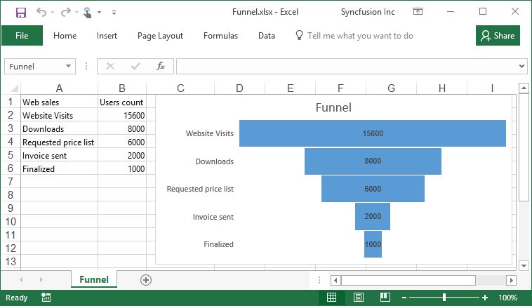
Box and Whisker
Box and Whisker chart shows distribution of data into quartiles, highlighting the mean and outliers. Box and Whisker charts are most commonly used in statistical analysis.
Following code example illustrates how to create Box and Whisker chart.
using (ExcelEngine excelEngine = new ExcelEngine())
{
  IApplication application = excelEngine.Excel;
  application.DefaultVersion = ExcelVersion.Excel2016;
  FileStream inputStream = new FileStream("Sample.xlsx", FileMode.Open, FileAccess.Read);
  IWorkbook workbook = application.Workbooks.Open(inputStream, ExcelOpenType.Automatic);
  IWorksheet sheet = workbook.Worksheets[0];

  //Create a chart
  IChartShape chart = sheet.Charts.Add();

  //Set the chart title
  chart.ChartTitle = "Test Scores";

  //Set chart type as Box and Whisker
  chart.ChartType = ExcelChartType.BoxAndWhisker;

  //Set data range in the worksheet
  chart.DataRange = sheet["A1:D16"];

  //Box and Whisker settings on first series
  IChartSerie seriesA = chart.Series[0];
  seriesA.SerieFormat.ShowInnerPoints = false;
  seriesA.SerieFormat.ShowOutlierPoints = true;
  seriesA.SerieFormat.ShowMeanMarkers = true;
  seriesA.SerieFormat.ShowMeanLine = false;
  seriesA.SerieFormat.QuartileCalculationType = ExcelQuartileCalculation.ExclusiveMedian;

  //Box and Whisker settings on second series
  IChartSerie seriesB = chart.Series[1];
  seriesB.SerieFormat.ShowInnerPoints = false;
  seriesB.SerieFormat.ShowOutlierPoints = true;
  seriesB.SerieFormat.ShowMeanMarkers = true;
  seriesB.SerieFormat.ShowMeanLine = false;
  seriesB.SerieFormat.QuartileCalculationType = ExcelQuartileCalculation.InclusiveMedian;

  //Box and Whisker settings on third series
  IChartSerie seriesC = chart.Series[2];
  seriesC.SerieFormat.ShowInnerPoints = false;
  seriesC.SerieFormat.ShowOutlierPoints = true;
  seriesC.SerieFormat.ShowMeanMarkers = true;
  seriesC.SerieFormat.ShowMeanLine = false;
  seriesC.SerieFormat.QuartileCalculationType = ExcelQuartileCalculation.ExclusiveMedian;

  //Saving the workbook as stream
  FileStream stream = new FileStream("Box and Whisker.xlsx", FileMode.Create, FileAccess.ReadWrite);
  workbook.SaveAs(stream);
  stream.Dispose();
}
using (ExcelEngine excelEngine = new ExcelEngine())
{
IApplication application = excelEngine.Excel;
application.DefaultVersion = ExcelVersion.Excel2016;
IWorkbook workbook = application.Workbooks.Open("Sample.xlsx", ExcelOpenType.Automatic);
IWorksheet sheet = workbook.Worksheets[0];
//Create a chart
IChartShape chart = sheet.Charts.Add();
//Set the chart title
chart.ChartTitle = "Test Scores";
//Set chart type as Box and Whisker
chart.ChartType = ExcelChartType.BoxAndWhisker;
//Set data range in the worksheet
chart.DataRange = sheet["A1:D16"];
//Box and Whisker settings on first series
IChartSerie seriesA = chart.Series[0];
seriesA.SerieFormat.ShowInnerPoints = false;
seriesA.SerieFormat.ShowOutlierPoints = true;
seriesA.SerieFormat.ShowMeanMarkers = true;
seriesA.SerieFormat.ShowMeanLine = false;
seriesA.SerieFormat.QuartileCalculationType = ExcelQuartileCalculation.ExclusiveMedian;
//Box and Whisker settings on second series
IChartSerie seriesB = chart.Series[1];
seriesB.SerieFormat.ShowInnerPoints = false;
seriesB.SerieFormat.ShowOutlierPoints = true;
seriesB.SerieFormat.ShowMeanMarkers = true;
seriesB.SerieFormat.ShowMeanLine = false;
seriesB.SerieFormat.QuartileCalculationType = ExcelQuartileCalculation.InclusiveMedian;
//Box and Whisker settings on third series
IChartSerie seriesC = chart.Series[2];
seriesC.SerieFormat.ShowInnerPoints = false;
seriesC.SerieFormat.ShowOutlierPoints = true;
seriesC.SerieFormat.ShowMeanMarkers = true;
seriesC.SerieFormat.ShowMeanLine = false;
seriesC.SerieFormat.QuartileCalculationType = ExcelQuartileCalculation.ExclusiveMedian;
workbook.SaveAs("Box and Whisker.xlsx");
}Using excelEngine As ExcelEngine = New ExcelEngine()
Dim application As IApplication = excelEngine.Excel
application.DefaultVersion = ExcelVersion.Excel2016
Dim workbook As IWorkbook = application.Workbooks.Open("Sample.xlsx", ExcelOpenType.Automatic)
Dim sheet As IWorksheet = workbook.Worksheets(0)
'Create a chart
Dim chart As IChartShape = sheet.Charts.Add()
'Set the chart title
chart.ChartTitle = "Test Scores"
'Set chart type as Box and Whisker
chart.ChartType = ExcelChartType.BoxAndWhisker
'Set data range in the worksheet
chart.DataRange = sheet("A1:D16")
'Box and Whisker settings on first series
Dim seriesA As IChartSerie = chart.Series(0)
seriesA.SerieFormat.ShowInnerPoints = False
seriesA.SerieFormat.ShowOutlierPoints = True
seriesA.SerieFormat.ShowMeanMarkers = True
seriesA.SerieFormat.ShowMeanLine = False
seriesA.SerieFormat.QuartileCalculationType = ExcelQuartileCalculation.ExclusiveMedian
'Box and Whisker settings on second series
Dim seriesB As IChartSerie = chart.Series(1)
seriesB.SerieFormat.ShowInnerPoints = False
seriesB.SerieFormat.ShowOutlierPoints = True
seriesB.SerieFormat.ShowMeanMarkers = True
seriesB.SerieFormat.ShowMeanLine = False
seriesB.SerieFormat.QuartileCalculationType = ExcelQuartileCalculation.InclusiveMedian
'Box and Whisker settings on third series
Dim seriesC As IChartSerie = chart.Series(2)
seriesC.SerieFormat.ShowInnerPoints = False
seriesC.SerieFormat.ShowOutlierPoints = True
seriesC.SerieFormat.ShowMeanMarkers = True
seriesC.SerieFormat.ShowMeanLine = False
seriesC.SerieFormat.QuartileCalculationType = ExcelQuartileCalculation.ExclusiveMedian
workbook.SaveAs("Box and Whisker.xlsx")
End UsingThe input template can be downloaded here.
A complete working example to create box and whisker chart in C# is present on this GitHub page.
The following screen shot shows the output of above code.
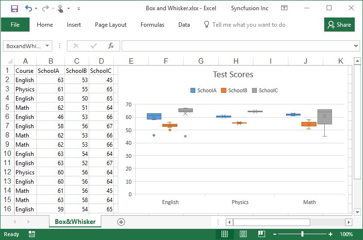
Waterfall
Waterfall chart helps to quickly understand the finances of business owners by viewing profit and loss statements. With a Waterfall chart, you can quickly illustrate the line items in your financial data and get a clear picture of how each item is impacting your bottom line.
Following code example illustrates how to create Waterfall chart.
using (ExcelEngine excelEngine = new ExcelEngine())
{
  IApplication application = excelEngine.Excel;
  application.DefaultVersion = ExcelVersion.Excel2016;
  FileStream inputStream = new FileStream("Sample.xlsx", FileMode.Open, FileAccess.Read);
  IWorkbook workbook = application.Workbooks.Open(inputStream,ExcelOpenType.Automatic);
  IWorksheet sheet = workbook.Worksheets[0];

  //Create a chart
  IChartShape chart = sheet.Charts.Add();

  //Set chart type as Waterfall
  chart.ChartType = ExcelChartType.WaterFall;

  //Set data range in the worksheet
  chart.DataRange = sheet["A2:B8"];

  //Data point settings as total in chart
  chart.Series[0].DataPoints[3].SetAsTotal = true;
  chart.Series[0].DataPoints[6].SetAsTotal = true;

  //Showing the connector lines between data points
  chart.Series[0].SerieFormat.ShowConnectorLines = true;

  //Set the chart title
  chart.ChartTitle = "Company Profit (in USD)";

  //Formatting data label and legend option
  chart.Series[0].DataPoints.DefaultDataPoint.DataLabels.IsValue = true;
  chart.Series[0].DataPoints.DefaultDataPoint.DataLabels.Size = 8;
  chart.Legend.Position = ExcelLegendPosition.Right;

  //Saving the workbook as stream
  FileStream stream = new FileStream("Waterfall.xlsx", FileMode.Create, FileAccess.ReadWrite);
  workbook.SaveAs(stream);
  stream.Dispose();
}
using (ExcelEngine excelEngine = new ExcelEngine())
{
IApplication application = excelEngine.Excel;
application.DefaultVersion = ExcelVersion.Excel2016;
IWorkbook workbook = application.Workbooks.Open("Sample.xlsx", ExcelOpenType.Automatic);
IWorksheet sheet = workbook.Worksheets[0];
//Create a chart
IChartShape chart = sheet.Charts.Add();
//Set chart type as Waterfall
chart.ChartType = ExcelChartType.WaterFall;
//Set data range in the worksheet
chart.DataRange = sheet["A2:B8"];
//Data point settings as total in chart
chart.Series[0].DataPoints[3].SetAsTotal = true;
chart.Series[0].DataPoints[6].SetAsTotal = true;
//Showing the connector lines between data points
chart.Series[0].SerieFormat.ShowConnectorLines = true;
//Set the chart title
chart.ChartTitle = "Company Profit (in USD)";
//Formatting data label and legend option
chart.Series[0].DataPoints.DefaultDataPoint.DataLabels.IsValue = true;
chart.Series[0].DataPoints.DefaultDataPoint.DataLabels.Size = 8;
chart.Legend.Position = ExcelLegendPosition.Right;
workbook.SaveAs("Waterfall.xlsx");
}Using excelEngine As ExcelEngine = New ExcelEngine()
Dim application As IApplication = excelEngine.Excel
application.DefaultVersion = ExcelVersion.Excel2016
Dim workbook As IWorkbook = application.Workbooks.Open("Sample.xlsx", ExcelOpenType.Automatic)
Dim sheet As IWorksheet = workbook.Worksheets(0)
'Create a chart
Dim chart As IChartShape = sheet.Charts.Add()
'Set chart type as Waterfall
chart.ChartType = ExcelChartType.WaterFall
'Set data range in the worksheet
chart.DataRange = sheet("A2:B8")
'Datapoint settings as total in chart
chart.Series(0).DataPoints(3).SetAsTotal = True
chart.Series(0).DataPoints(6).SetAsTotal = True
'Showing the connector lines between data points
chart.Series(0).SerieFormat.ShowConnectorLines = True
'Set the chart title
chart.ChartTitle = "Company Profit (in USD)"
'Formatting data label and legend option
chart.Series(0).DataPoints.DefaultDataPoint.DataLabels.IsValue = True
chart.Series(0).DataPoints.DefaultDataPoint.DataLabels.Size = 8
chart.Legend.Position = ExcelLegendPosition.Right
workbook.SaveAs("Waterfall.xlsx")
End UsingThe input template can be downloaded here.
A complete working example to create waterfall chart in C# is present on this GitHub page.
The following screen shot shows the output of above code.
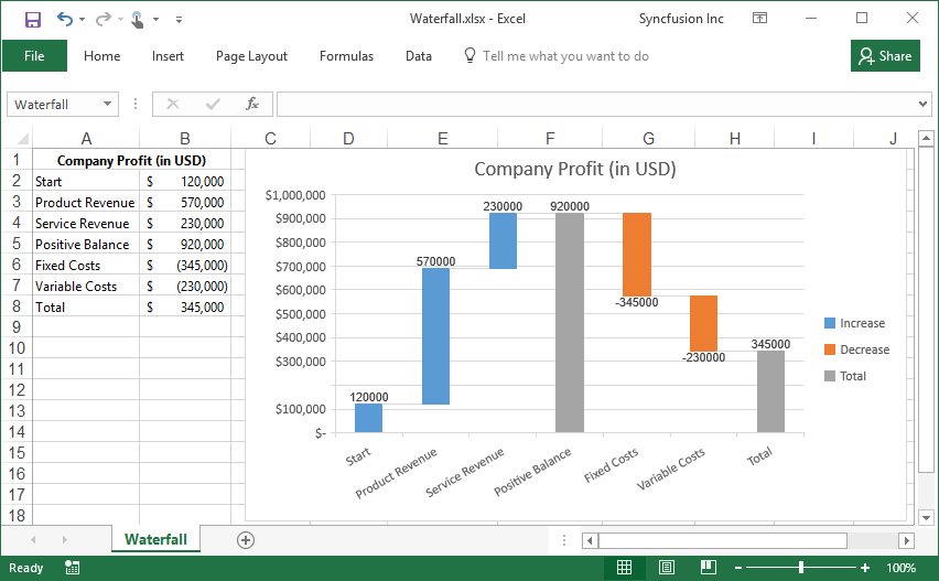
Histogram
Histogram shows the frequencies within a distribution. Each column of the chart is called a bin, which can be changed further to analyze the data.
Following code example illustrates how to create Histogram.
using (ExcelEngine excelEngine = new ExcelEngine())
{
  IApplication application = excelEngine.Excel;
  application.DefaultVersion = ExcelVersion.Excel2016;
  FileStream inputStream = new FileStream("Sample.xlsx", FileMode.Open, FileAccess.Read);
  IWorkbook workbook = application.Workbooks.Open(inputStream, ExcelOpenType.Automatic);
  IWorksheet sheet = workbook.Worksheets[0];

  //Create a chart
  IChartShape chart = sheet.Charts.Add();

  //Set chart type as Histogram
  chart.ChartType = ExcelChartType.Histogram;

  //Set data range in the worksheet
  chart.DataRange = sheet["A1:A15"];

  //Category axis bin settings
  chart.PrimaryCategoryAxis.BinWidth = 8;

  //Gap width settings
  chart.Series[0].SerieFormat.CommonSerieOptions.GapWidth = 6;

  //Set the chart title and axis title
  chart.ChartTitle = "Height Data";
  chart.PrimaryValueAxis.Title = "Number of students";
  chart.PrimaryCategoryAxis.Title = "Height";

  //Hiding the legend
  chart.HasLegend = false;

  //Saving the workbook as stream
  FileStream stream = new FileStream("Histogram.xlsx", FileMode.Create, FileAccess.ReadWrite);
  workbook.SaveAs(stream);
  stream.Dispose();
}
using (ExcelEngine excelEngine = new ExcelEngine())
{
IApplication application = excelEngine.Excel;
application.DefaultVersion = ExcelVersion.Excel2016;
IWorkbook workbook = application.Workbooks.Open("Sample.xlsx", ExcelOpenType.Automatic);
IWorksheet sheet = workbook.Worksheets[0];
//Create a chart
IChartShape chart = sheet.Charts.Add();
//Set chart type as Histogram
chart.ChartType = ExcelChartType.Histogram;
//Set data range in the worksheet
chart.DataRange = sheet["A1:A15"];
//Category axis bin settings
chart.PrimaryCategoryAxis.BinWidth = 8;
//Gap width settings
chart.Series[0].SerieFormat.CommonSerieOptions.GapWidth = 6;
//Set the chart title and axis title
chart.ChartTitle = "Height Data";
chart.PrimaryValueAxis.Title = "Number of students";
chart.PrimaryCategoryAxis.Title = "Height";
//Hiding the legend
chart.HasLegend = false;
workbook.SaveAs("Histogram.xlsx");
}Using excelEngine As ExcelEngine = New ExcelEngine()
Dim application As IApplication = excelEngine.Excel
application.DefaultVersion = ExcelVersion.Excel2016
Dim workbook As IWorkbook = application.Workbooks.Open("Sample.xlsx", ExcelOpenType.Automatic)
Dim sheet As IWorksheet = workbook.Worksheets(0)
'Create a chart
Dim chart As IChartShape = sheet.Charts.Add()
'Set chart type as Histogram
chart.ChartType = ExcelChartType.Histogram
'Set data range in the worksheet
chart.DataRange = sheet("A1:A15")
'Category axis bin settings
chart.PrimaryCategoryAxis.BinWidth = 8
'Gap width settings
chart.Series(0).SerieFormat.CommonSerieOptions.GapWidth = 6
'Set the chart title and axis title
chart.ChartTitle = "Height Data"
chart.PrimaryValueAxis.Title = "Number of students"
chart.PrimaryCategoryAxis.Title = "Height"
'Hiding the legend
chart.HasLegend = False
workbook.SaveAs("Histogram.xlsx")
End UsingThe input template can be downloaded here.
A complete working example to create histogram chart in C# is present on this GitHub page.
The following screen shot shows the output of above code.
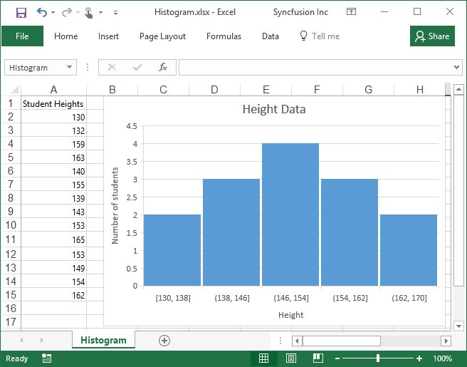
Pareto
Pareto is a sorted histogram where columns sorted in descending order and a line representing the cumulative total percentage.
Following code example illustrates how to create Pareto chart.
using (ExcelEngine excelEngine = new ExcelEngine())
{
  IApplication application = excelEngine.Excel;
  application.DefaultVersion = ExcelVersion.Excel2016;
  FileStream inputStream = new FileStream("Sample.xlsx", FileMode.Open, FileAccess.Read);
  IWorkbook workbook = application.Workbooks.Open(inputStream, ExcelOpenType.Automatic);
  IWorksheet sheet = workbook.Worksheets[0];

  //Create a chart
  IChartShape chart = sheet.Charts.Add();

  //Set chart type as Pareto
  chart.ChartType = ExcelChartType.Pareto;

  //Set data range in the worksheet
  chart.DataRange = sheet["A2:B8"];

  //Set category values as bin values
  chart.PrimaryCategoryAxis.IsBinningByCategory = true;

  //Formatting Pareto line
  chart.Series[0].ParetoLineFormat.LineProperties.ColorIndex = ExcelKnownColors.Bright_green;

  //Gap width settings
  chart.Series[0].SerieFormat.CommonSerieOptions.GapWidth = 6;

  //Set the chart title
  chart.ChartTitle = "Expenses";

  //Hiding the legend
  chart.HasLegend = false;

  //Saving the workbook as stream
  FileStream stream = new FileStream("Pareto.xlsx", FileMode.Create, FileAccess.ReadWrite);
  workbook.SaveAs(stream);
  stream.Dispose();
}
using (ExcelEngine excelEngine = new ExcelEngine())
{
IApplication application = excelEngine.Excel;
application.DefaultVersion = ExcelVersion.Excel2016;
IWorkbook workbook = application.Workbooks.Open("Sample.xlsx", ExcelOpenType.Automatic);
IWorksheet sheet = workbook.Worksheets[0];
//Create a chart
IChartShape chart = sheet.Charts.Add();
//Set chart type as Pareto
chart.ChartType = ExcelChartType.Pareto;
//Set data range in the worksheet
chart.DataRange = sheet["A2:B8"];
//Set category values as bin values
chart.PrimaryCategoryAxis.IsBinningByCategory = true;
//Formatting Pareto line
chart.Series[0].ParetoLineFormat.LineProperties.ColorIndex = ExcelKnownColors.Bright_green;
//Gap width settings
chart.Series[0].SerieFormat.CommonSerieOptions.GapWidth = 6;
//Set the chart title
chart.ChartTitle = "Expenses";
//Hiding the legend
chart.HasLegend = false;
workbook.SaveAs("Pareto.xlsx");
}Using excelEngine As ExcelEngine = New ExcelEngine()
Dim application As IApplication = excelEngine.Excel
application.DefaultVersion = ExcelVersion.Excel2016
Dim workbook As IWorkbook = application.Workbooks.Open("Sample.xlsx", ExcelOpenType.Automatic)
Dim sheet As IWorksheet = workbook.Worksheets(0)
'Create a chart
Dim chart As IChartShape = sheet.Charts.Add()
'Set chart type as Pareto
chart.ChartType = ExcelChartType.Pareto
'Set data range in the worksheet
chart.DataRange = sheet("A2:B8")
'Set category axis as bin option
chart.PrimaryCategoryAxis.IsBinningByCategory = True
'Formatting Pareto line
chart.Series(0).ParetoLineFormat.LineProperties.ColorIndex = ExcelKnownColors.Bright_green
'Gap width settings
chart.Series(0).SerieFormat.CommonSerieOptions.GapWidth = 6
'Set the chart title
chart.ChartTitle = "Expenses"
'Hiding the legend
chart.HasLegend = False
workbook.SaveAs("Pareto.xlsx")
End UsingThe input template can be downloaded here.
A complete working example to create pareto chart in C# is present on this GitHub page.
The following screen shot shows the output of above code.
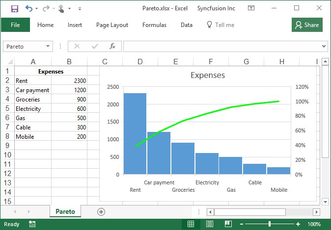
Treemap
Treemap provides a hierarchical view of data as clustered rectangle with a specific weighted attribute determining the size of the rectangle.
Following code example illustrates how to create Treemap chart.
using (ExcelEngine excelEngine = new ExcelEngine())
{
  IApplication application = excelEngine.Excel;
  application.DefaultVersion = ExcelVersion.Excel2016;
  FileStream inputStream = new FileStream("Sample.xlsx", FileMode.Open, FileAccess.Read);
  IWorkbook workbook = application.Workbooks.Open(inputStream, ExcelOpenType.Automatic);
  IWorksheet sheet = workbook.Worksheets[0];

  //Create a chart
  IChartShape chart = sheet.Charts.Add();

  //Set chart type as TreeMap
  chart.ChartType = ExcelChartType.TreeMap;

  //Set data range in the worksheet
  chart.DataRange = sheet["A2:C11"];

  //Set the chart title
  chart.ChartTitle = "Area by countries";

  //Set the Treemap label option
  chart.Series[0].SerieFormat.TreeMapLabelOption = ExcelTreeMapLabelOption.Banner;

  //Formatting data labels
  chart.Series[0].DataPoints.DefaultDataPoint.DataLabels.Size = 8;

  //Saving the workbook as stream
  FileStream stream = new FileStream("Treemap.xlsx", FileMode.Create, FileAccess.ReadWrite);
  workbook.SaveAs(stream);
  stream.Dispose();
}
using (ExcelEngine excelEngine = new ExcelEngine())
{
IApplication application = excelEngine.Excel;
application.DefaultVersion = ExcelVersion.Excel2016;
IWorkbook workbook = application.Workbooks.Open("Sample.xlsx", ExcelOpenType.Automatic);
IWorksheet sheet = workbook.Worksheets[0];
//Create a chart
IChartShape chart = sheet.Charts.Add();
//Set chart type as TreeMap
chart.ChartType = ExcelChartType.TreeMap;
//Set data range in the worksheet
chart.DataRange = sheet["A2:C11"];
//Set the chart title
chart.ChartTitle = "Area by countries";
//Set the Treemap label option
chart.Series[0].SerieFormat.TreeMapLabelOption = ExcelTreeMapLabelOption.Banner;
//Formatting data labels
chart.Series[0].DataPoints.DefaultDataPoint.DataLabels.Size = 8;
workbook.SaveAs("Treemap.xlsx");
}Using excelEngine As ExcelEngine = New ExcelEngine()
Dim application As IApplication = excelEngine.Excel
application.DefaultVersion = ExcelVersion.Excel2016
Dim workbook As IWorkbook = application.Workbooks.Open("Sample.xlsx", ExcelOpenType.Automatic)
Dim sheet As IWorksheet = workbook.Worksheets(0)
'Create a chart
Dim chart As IChartShape = sheet.Charts.Add()
'Set chart type as TreeMap
chart.ChartType = ExcelChartType.TreeMap
'Set data range in the worksheet
chart.DataRange = sheet("A2:C11")
'Set the chart title
chart.ChartTitle = "Area by countries"
'Set the Treemap label option
chart.Series(0).SerieFormat.TreeMapLabelOption = ExcelTreeMapLabelOption.Banner
'Formatting data labels
chart.Series(0).DataPoints.DefaultDataPoint.DataLabels.Size = 8
workbook.SaveAs("Treemap.xlsx")
End UsingThe input template can be downloaded here.
A complete working example to create treemap chart in C# is present on this GitHub page.
The following screen shot shows the output of above code.
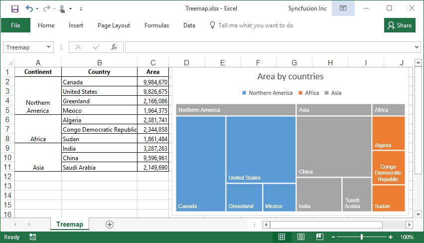
Sunburst
Sunburst provides a hierarchical view of data where each level of the hierarchy is represented by one ring or circle with the innermost circle as the top of the hierarchy.
Following code example illustrates how to create Sunburst chart.
using (ExcelEngine excelEngine = new ExcelEngine())
{
  IApplication application = excelEngine.Excel;
  application.DefaultVersion = ExcelVersion.Excel2016;
  FileStream inputStream = new FileStream("Sample.xlsx", FileMode.Open, FileAccess.Read);
  IWorkbook workbook = application.Workbooks.Open(inputStream, ExcelOpenType.Automatic);
  IWorksheet sheet = workbook.Worksheets[0];

  //Create a chart
  IChartShape chart = sheet.Charts.Add();

  //Set chart type as Sunburst
  chart.ChartType = ExcelChartType.SunBurst;

  //Set data range in the worksheet
  chart.DataRange = sheet["A1:D16"];

  //Set the chart title
  chart.ChartTitle = "Sales by annual";

  //Formatting data labels
  chart.Series[0].DataPoints.DefaultDataPoint.DataLabels.Size = 8;

  //Hiding the legend
  chart.HasLegend = false;

  //Saving the workbook as stream
  FileStream stream = new FileStream("Sunburst.xlsx", FileMode.Create, FileAccess.ReadWrite);
  workbook.SaveAs(stream);
  stream.Dispose();
}
using (ExcelEngine excelEngine = new ExcelEngine())
{
IApplication application = excelEngine.Excel;
application.DefaultVersion = ExcelVersion.Excel2016;
IWorkbook workbook = application.Workbooks.Open("Sample.xlsx", ExcelOpenType.Automatic);
IWorksheet sheet = workbook.Worksheets[0];
//Create a chart
IChartShape chart = sheet.Charts.Add();
//Set chart type as Sunburst
chart.ChartType = ExcelChartType.SunBurst;
//Set data range in the worksheet
chart.DataRange = sheet["A1:D16"];
//Set the chart title
chart.ChartTitle = "Sales by annual";
//Formatting data labels
chart.Series[0].DataPoints.DefaultDataPoint.DataLabels.Size = 8;
//Hiding the legend
chart.HasLegend = false;
workbook.SaveAs("Sunburst.xlsx");
}Using excelEngine As ExcelEngine = New ExcelEngine()
Dim application As IApplication = excelEngine.Excel
application.DefaultVersion = ExcelVersion.Excel2016
Dim workbook As IWorkbook = application.Workbooks.Open("Sample.xlsx", ExcelOpenType.Automatic)
Dim sheet As IWorksheet = workbook.Worksheets(0)
'Create a chart
Dim chart As IChartShape = sheet.Charts.Add()
'Set chart type as Sunburst
chart.ChartType = ExcelChartType.SunBurst
'Set data range in the worksheet
chart.DataRange = sheet("A1:D16")
'Set the chart title
chart.ChartTitle = "Sales by annual"
'Formatting data labels
chart.Series(0).DataPoints.DefaultDataPoint.DataLabels.Size = 8
'Hiding the legend
chart.HasLegend = False
workbook.SaveAs("Sunburst.xlsx")
End UsingThe input template can be downloaded here.
A complete working example to create sunburst chart in C# is present on this GitHub page.
The following screen shot shows the output of above code.
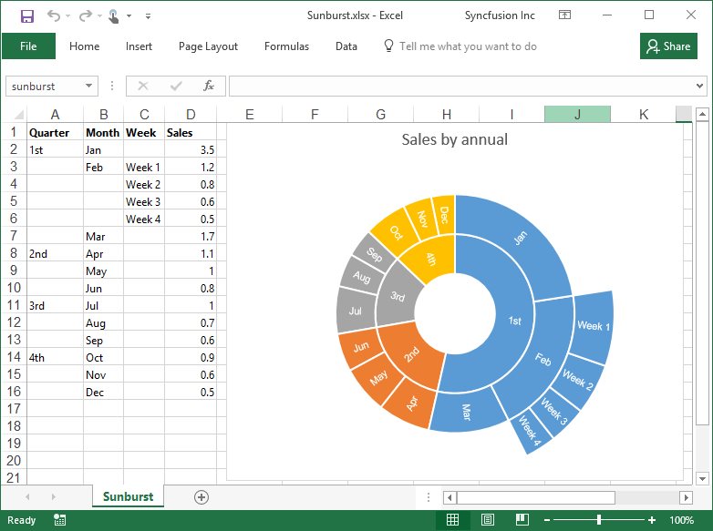
NOTE
These Charts are supported only in Excel 2016 and are not visible in the earlier versions.
Supported Chart Types
The following chart types are supported in XlsIO.
- Area
- Area_3D
- Area_Stacked
- Area_Stacked_100
- Area_Stacked_100_3D
- Area_Stacked_3D
- Bar_Clustered
- Bar_Clustered_3D
- Bar_Stacked
- Bar_Stacked_100
- Bar_Stacked_100_3D
- Bar_Stacked_3D
- Bubble
- Bubble_3D
- Column_3D
- Column_Clustered
- Column_Clustered_3D
- Column_Stacked
- Column_Stacked_100
- Column_Stacked_100_3D
- Column_Stacked_3D
- Combination_Chart
- Cone_Bar_Clustered
- Cone_Bar_Stacked
- Cone_Bar_Stacked_100
- Cone_Clustered
- Cone_Clustered_3D
- Cone_Stacked
- Cone_Stacked_100
- Cylinder_Bar_Clustered
- Cylinder_Bar_Stacked
- Cylinder_Bar_Stacked_100
- Cylinder_Clustered
- Cylinder_Clustered_3D
- Cylinder_Stacked
- Cylinder_Stacked_100
- Doughnut
- Doughnut_Exploded
- Line
- Line_3D
- Line_Markers
- Line_Markers_Stacked
- Line_Markers_Stacked_100
- Line_Stacked
- Line_Stacked_100
- Pie
- Pie_3D
- Pie_Bar
- Pie_Exploded
- Pie_Exploded_3D
- PieOfPie
- Pyramid_Bar_Clustered
- Pyramid_Bar_Stacked
- Pyramid_Bar_Stacked_100
- Pyramid_Clustered
- Pyramid_Clustered_3D
- Pyramid_Stacked
- Pyramid_Stacked_100
- Radar
- Radar_Filled
- Radar_Markers
- Scatter_Line
- Scatter_Line_Markers
- Scatter_Markers
- Scatter_SmoothedLine
- Scatter_SmoothedLine_Markers
- Stock_HighLowClose
- Stock_OpenHighLowClose
- Stock_VolumeHighLowClose
- Stock_VolumeOpenHighLowClose
- Surface_3D
- Surface_Contour
- Surface_NoColor_3D
- Surface_NoColor_Contour
- Funnel
- Box and Whisker
- Waterfall
- Histogram
- Pareto
- Treemap
- Sunburst