Formatting in Vue Spreadsheet

28 Sep 202624 minutes to read

Formatting options make your data easier to view and understand. The Spreadsheet supports the following types of formatting:

• Number Formatting
• Text Formatting
• Cell Formatting
• Conditional Formatting
• Rich Text Formatting

Number Formatting

Number formatting provides a type for your data in the Spreadsheet. Use the allowNumberFormatting property to enable or disable the number formatting option in the Spreadsheet. The default value of allowNumberFormatting is true. The types of number formatting supported in the Spreadsheet are:

Types	Format Code	Format ID
General(default)	NA	0
Number	0.00	2
Currency	$#,##0.00	NA
Accounting	_($* #,##0.00_);_($* (#,##0.00);_($* "-"??_);_(@_)	44
ShortDate	m/d/yyyy	14
LongDate	dddd, mmmm dd, yyyy	NA
Time	h:mm:ss AM/PM	NA
Percentage	0.00%	10
Fraction	# ?/?	12
Scientific	0.00E+00	11
Text	@	49

Number formatting can be applied in the following ways:

• Using the format property in cell, you can set the desired format to each cell at initial load.
• Using the numberFormat method to set the number format on a cell or range of cells.
• Select the number format option from the ribbon toolbar.

The following code example shows the number formatting in cell data.

Composition API (~/src/App.vue)

<template>
  <ejs-spreadsheet ref="spreadsheet" :created="created" :showFormulaBar="false" :showRibbon="false"
    :showSheetTabs="false" :allowInsert="false" :allowDelete="false">
    <e-sheets>
      <e-sheet :showGridLines="false">
        <e-ranges>
          <e-range :dataSource="dataSource" startCell="A2"></e-range>
        </e-ranges>
        <e-columns>
          <e-column :width=140></e-column>
          <e-column :width=140></e-column>
          <e-column :width=160></e-column>
          <e-column :width=160></e-column>
          <e-column :width=160></e-column>
          <e-column :width=120></e-column>
        </e-columns>
        <e-rows>
          <e-row :height=35 customHeight="true">
            <e-cells>
              <e-cell value="Sales Team Summary" colSpan=6></e-cell>
            </e-cells>
          </e-row>
          <e-row :index=10>
            <e-cells>
              <e-cell index=1 value="Total:"></e-cell>
              <e-cell formula="=SUM(C3:C10)" format="$#,##0.00"></e-cell>
              <e-cell formula="=SUM(D3:D10)" format='_($* #,##0.00_);_($* (#,##0.00);_($* "-"??_);_(@_)'></e-cell>
              <e-cell formula="=SUM(E3:E10)" format='_($* #,##0.00_);_($* (#,##0.00);_($* "-"??_);_(@_)'></e-cell>
            </e-cells>
          </e-row>
        </e-rows>
      </e-sheet>
    </e-sheets>
  </ejs-spreadsheet>
</template>

<script setup>
import { ref } from "vue";
import { SpreadsheetComponent as EjsSpreadsheet, ColumnsDirective as EColumns, ColumnDirective as EColumn, RowsDirective as ERows, RowDirective as ERow, CellsDirective as ECells, CellDirective as ECell, RangesDirective as ERanges, RangeDirective as ERange, SheetsDirective as ESheets, SheetDirective as ESheet } from "@syncfusion/ej2-vue-spreadsheet";
import { data } from './data.js';

const spreadsheet = ref(null);
const dataSource = data;

const created = function () {
  spreadsheet.value.cellFormat({
    fontWeight: 'bold', fontSize: '12pt', backgroundColor: '#279377', textAlign: 'center',
    color: '#ffffff', borderBottom: '1px solid #e0e0e0'
  }, 'A2:F2');
  spreadsheet.value.cellFormat({ borderTop: '1px solid #e0e0e0', backgroundColor: '#EEEEEE' }, 'A11:F11');
  spreadsheet.value.cellFormat({ fontWeight: 'bold', fontStyle: 'italic' }, 'B11');
  spreadsheet.value.cellFormat({ verticalAlign: 'middle', textAlign: 'center', fontSize: '16pt', fontWeight: 'bold', border: '1px solid #e0e0e0', backgroundColor: '#EEEEEE', color: '#279377' }, 'A1');
  spreadsheet.value.setBorder({ border: '1px solid #e0e0e0' }, 'A2:F11', 'Outer');
  // Applied Accounting format to the cells from C3 to E10 range.
  spreadsheet.value.numberFormat('_($* #,##0.00_);_($* (#,##0.00);_($* "-"??_);_(@_)', 'C3:E10');
  // Applied Percentage format to the cells from C3 to E11 range.
  spreadsheet.value.numberFormat('0%', 'F3:F10');
}
</script>
<style>
@import '../node_modules/@syncfusion/ej2-base/styles/tailwind3.css';
@import '../node_modules/@syncfusion/ej2-buttons/styles/tailwind3.css';
@import '../node_modules/@syncfusion/ej2-dropdowns/styles/tailwind3.css';
@import '../node_modules/@syncfusion/ej2-inputs/styles/tailwind3.css';
@import '../node_modules/@syncfusion/ej2-navigations/styles/tailwind3.css';
@import '../node_modules/@syncfusion/ej2-popups/styles/tailwind3.css';
@import '../node_modules/@syncfusion/ej2-splitbuttons/styles/tailwind3.css';
@import '../node_modules/@syncfusion/ej2-grids/styles/tailwind3.css';
@import "../node_modules/@syncfusion/ej2-vue-spreadsheet/styles/tailwind3.css";
</style>

Options API (~/src/App.vue)

<template>
  <ejs-spreadsheet ref="spreadsheet" :created="created" :showFormulaBar="false" :showRibbon="false"
    :showSheetTabs="false" :allowInsert="false" :allowDelete="false">
    <e-sheets>
      <e-sheet :showGridLines="false">
        <e-ranges>
          <e-range :dataSource="dataSource" startCell="A2"></e-range>
        </e-ranges>
        <e-columns>
          <e-column :width=140></e-column>
          <e-column :width=140></e-column>
          <e-column :width=160></e-column>
          <e-column :width=160></e-column>
          <e-column :width=160></e-column>
          <e-column :width=120></e-column>
        </e-columns>
        <e-rows>
          <e-row :height=35 customHeight="true">
            <e-cells>
              <e-cell value="Sales Team Summary" colSpan=6></e-cell>
            </e-cells>
          </e-row>
          <e-row :index=10>
            <e-cells>
              <e-cell index=1 value="Total:"></e-cell>
              <e-cell formula="=SUM(C3:C10)" format="$#,##0.00"></e-cell>
              <e-cell formula="=SUM(D3:D10)" format='_($* #,##0.00_);_($* (#,##0.00);_($* "-"??_);_(@_)'></e-cell>
              <e-cell formula="=SUM(E3:E10)" format='_($* #,##0.00_);_($* (#,##0.00);_($* "-"??_);_(@_)'></e-cell>
            </e-cells>
          </e-row>
        </e-rows>
      </e-sheet>
    </e-sheets>
  </ejs-spreadsheet>
</template>

<script>
import { SpreadsheetComponent, ColumnsDirective, ColumnDirective, RowsDirective, RowDirective, CellsDirective, CellDirective, RangesDirective, RangeDirective, SheetsDirective, SheetDirective } from "@syncfusion/ej2-vue-spreadsheet";
import { data } from './data.js';

export default {
  name: "App",
  components: {
    "ejs-spreadsheet": SpreadsheetComponent,
    "e-sheets": SheetsDirective,
    "e-sheet": SheetDirective,
    "e-ranges": RangesDirective,
    "e-range": RangeDirective,
    "e-columns": ColumnsDirective,
    "e-column": ColumnDirective,
    "e-rows": RowsDirective,
    "e-row": RowDirective,
    "e-cells": CellsDirective,
    "e-cell": CellDirective
  },
  data: () => {
    return {
      dataSource: data
    }
  },
  methods: {
    created: function () {
      let spreadsheet = this.$refs.spreadsheet;
      spreadsheet.cellFormat({
        fontWeight: 'bold', fontSize: '12pt', backgroundColor: '#279377', textAlign: 'center',
        color: '#ffffff', borderBottom: '1px solid #e0e0e0'
      }, 'A2:F2');
      spreadsheet.cellFormat({ borderTop: '1px solid #e0e0e0', backgroundColor: '#EEEEEE' }, 'A11:F11');
      spreadsheet.cellFormat({ fontWeight: 'bold', fontStyle: 'italic' }, 'B11');
      spreadsheet.cellFormat({ verticalAlign: 'middle', textAlign: 'center', fontSize: '16pt', fontWeight: 'bold', border: '1px solid #e0e0e0', backgroundColor: '#EEEEEE', color: '#279377' }, 'A1');
      spreadsheet.setBorder({ border: '1px solid #e0e0e0' }, 'A2:F11', 'Outer');
      // Applied Accounting format to the cells from C3 to E10 range.
      spreadsheet.numberFormat('_($* #,##0.00_);_($* (#,##0.00);_($* "-"??_);_(@_)', 'C3:E10');
      // Applied Percentage format to the cells from C3 to E11 range.
      spreadsheet.numberFormat('0%', 'F3:F10');
    }
  }
}
</script>
<style>
@import '../node_modules/@syncfusion/ej2-base/styles/tailwind3.css';
@import '../node_modules/@syncfusion/ej2-buttons/styles/tailwind3.css';
@import '../node_modules/@syncfusion/ej2-dropdowns/styles/tailwind3.css';
@import '../node_modules/@syncfusion/ej2-inputs/styles/tailwind3.css';
@import '../node_modules/@syncfusion/ej2-navigations/styles/tailwind3.css';
@import '../node_modules/@syncfusion/ej2-popups/styles/tailwind3.css';
@import '../node_modules/@syncfusion/ej2-splitbuttons/styles/tailwind3.css';
@import '../node_modules/@syncfusion/ej2-grids/styles/tailwind3.css';
@import "../node_modules/@syncfusion/ej2-vue-spreadsheet/styles/tailwind3.css";
</style>

Limitations of Number Formatting

• Custom number formatting is not supported.

Configure culture-based custom format

Previously, the custom format dialog always displayed formats using the English settings (group separator, decimal separator, and currency symbol were not updated based on the applied culture). Starting from version 27.1.*, the custom format dialog will now display formats according to the applied culture. You can select a culture-based number format from the dialog or enter your own format using the culture-specific decimal separator, group separator, and currency symbol. Then, click “Apply” to apply the culture-specific custom format to the selected cells.

The spreadsheet allows customization of formats in the custom format dialog using the configureLocalizedFormat method. In this method, you need to pass a collection containing the default number format IDs and their corresponding format codes as arguments. Based on this collection, the custom format dialog will display the customized formats. You can refer to the default number format IDs from the Excel built-in number format reference.

Compared to Excel, the date, time, currency, and accounting formats vary across different cultures. For example, when an Excel file with the date format 'm/d/yyyy' is imported in the en-US culture, the spreadsheet displays the date in that format. However, when the same file is imported in the German culture, the date format changes to 'dd.MM.yyyy', which is the default for that region. The default number format ID for the date is 14. To customize the date format based on the culture, you should map the default number format ID to the appropriate culture-specific format code, like this: { id: 14, code: 'dd.MM.yyyy' } in the configureLocalizedFormat method.

The format code should use the default decimal separator (.) and group separator (,).

The code below illustrates how culture-based format codes are mapped to their corresponding number format ID for the German (de) culture.

import { configureLocalizedFormat } from "@syncfusion/ej2-vue-spreadsheet";

const deLocaleFormats = [
    { id: 14, code: 'dd.MM.yyyy' },
    { id: 15, code: 'dd. MMM yy' },
    { id: 16, code: 'dd. MMM' },
    { id: 17, code: 'MMM yy' },
    { id: 20, code: 'hh:mm' },
    { id: 21, code: 'hh:mm:ss' },
    { id: 22, code: 'dd.MM.yyyy hh:mm' },
    { id: 37, code: '#,##0;-#,##0' },
    { id: 38, code: '#,##0;[Red]-#,##0' },
    { id: 39, code: '#,##0.00;-#,##0.00' },
    { id: 40, code: '#,##0.00;[Red]-#,##0.00' },
    { id: 5, code: '#,##0 "€";-#,##0 "€"' },
    { id: 6, code: '#,##0 "€";[Red]-#,##0 "€"' },
    { id: 7, code: '#,##0.00 "€";-#,##0.00 "€"' },
    { id: 8, code: '#,##0.00 "€";[Red]-#,##0.00 "€"' },
    { id: 41, code: '_-* #,##0_-;-* #,##0_-;_-* "-"_-;_-@_-' },
    { id: 42, code: '_-* #,##0 "€"_-;-* #,##0 "€"_-;_-* "-" "€"_-;_-@_-' },
    { id: 43, code: '_-* #,##0.00_-;-* #,##0.00_-;_-* "-"??_-;_-@_-' },
    { id: 44, code: '_-* #,##0.00 "€"_-;-* #,##0.00 "€"_-;_-* "-"?? "€"_-;_-@_-' }
];

// Mapping culture-based number formats for the "de" culture: The "spreadsheet.ej2Instances" parameter is an instance of the spreadsheet component, and the "deLocaleFormats" parameter is an array containing format codes and their corresponding format IDs for the "de" culture.
configureLocalizedFormat(spreadsheet.ej2Instances, deLocaleFormats);

The following code example demonstrates how to configure culture-based formats for different cultures in the spreadsheet.

Composition API (~/src/App.vue)

<template>
  <div id="app">
    <ejs-dropdownlist id='ddlelement' :index='index' :width='width' :dataSource='cultureList' :fields='fields' :popupHeight='popupHeight' :placeholder='placeholder' :change="change"></ejs-dropdownlist>
    <ejs-spreadsheet ref="spreadsheet" locale="de" listSeparator=";" :created="created">
      <e-sheets>
        <e-sheet>
          <e-ranges>
            <e-range :dataSource="dataSource"></e-range>
          </e-ranges>
          <e-columns>
            <e-column :width=120></e-column>
            <e-column :width=180></e-column>
            <e-column :width=100></e-column>
            <e-column :width=120></e-column>
            <e-column :width=120></e-column>
          </e-columns>
        </e-sheet>
      </e-sheets>
    </ejs-spreadsheet>
  </div>
</template>
<script setup>
import { ref } from "vue";
import { SpreadsheetComponent as EjsSpreadsheet, ColumnsDirective as EColumns, ColumnDirective as EColumn,  RangesDirective as ERanges, RangeDirective as ERange, SheetsDirective as ESheets, SheetDirective as ESheet, getFormatFromType, configureLocalizedFormat } from "@syncfusion/ej2-vue-spreadsheet";
import { DropDownListComponent as EjsDropdownlist } from '@syncfusion/ej2-vue-dropdowns';
import { loadCldr, setCulture, setCurrencyCode, Ajax } from '@syncfusion/ej2-base';
import { data } from './datasource.js';

let loadCultureFiles = (locales) => {
let files = ['ca-gregorian', 'numbers', 'timeZoneNames', 'currencies', 'numberingSystems'];
  locales.forEach((locale) => {
    for (const fileName of files) {
      const url = `./cldr-data/${fileName === 'numberingSystems' ? '' : `${locale}/`}${fileName}.json`;
      const ajax = new Ajax(url, 'GET', false);
      ajax.onSuccess = (value) => loadCldr(JSON.parse(value));
      ajax.send();
    }
  });
}

loadCultureFiles(['de', 'fr-CH', 'zh']);
// Setting German culture.
setCulture('de');
// Setting currency code for the German culture.
setCurrencyCode('EUR');

let localeFormats = {
  'de': [{ id: 37, code: '#,##0;-#,##0' }, { id: 38, code: '#,##0;[Red]-#,##0' },
  { id: 39, code: '#,##0.00;-#,##0.00' }, { id: 40, code: '#,##0.00;[Red]-#,##0.00' }, { id: 5, code: '#,##0 "€";-#,##0 "€"' },
  { id: 6, code: '#,##0 "€";[Red]-#,##0 "€"' }, { id: 7, code: '#,##0.00 "€";-#,##0.00 "€"' },
  { id: 8, code: '#,##0.00 "€";[Red]-#,##0.00 "€"' }, { id: 41, code: '_-* #,##0_-;-* #,##0_-;_-* "-"_-;_-@_-' },
  { id: 42, code: '_-* #,##0 "€"_-;-* #,##0 "€"_-;_-* "-" "€"_-;_-@_-' },
  { id: 43, code: '_-* #,##0.00_-;-* #,##0.00_-;_-* "-"??_-;_-@_-' },
  { id: 44, code: '_-* #,##0.00 "€"_-;-* #,##0.00 "€"_-;_-* "-"?? "€"_-;_-@_-' },
  { id: 14, code: 'dd.MM.yyyy' }, { id: 15, code: 'dd. MMM yy' }, { id: 16, code: 'dd. MMM' }, { id: 17, code: 'MMM yy' },
  { id: 20, code: 'hh:mm' }, { id: 21, code: 'hh:mm:ss' }, { id: 22, code: 'dd.MM.yyyy hh:mm' }],
  'zh': [{ id: 37, code: '#,##0;-#,##0' }, { id: 38, code: '#,##0;[Red]-#,##0' }, { id: 39, code: '#,##0.00;-#,##0.00' },
  { id: 40, code: '#,##0.00;[Red]-#,##0.00' }, { id: 5, code: '"¥"#,##0;"¥"-#,##0' }, { id: 6, code: '"¥"#,##0;[Red]"¥"-#,##0' },
  { id: 7, code: '"¥"#,##0.00;"¥"-#,##0.00' }, { id: 8, code: '"¥"#,##0.00;[Red]"¥"-#,##0.00' },
  { id: 41, code: '_ * #,##0_ ;_ * -#,##0_ ;_ * "-"_ ;_ @_' }, { id: 42, code: '_ "¥"* #,##0_ ;_ "¥"* -#,##0_ ;_ "¥"* "-"_ ;_ @_' },
  { id: 43, code: '_ * #,##0.00_ ;_ * -#,##0.00_ ;_ * "-"??_ ;_ @_' },
  { id: 44, code: '_ "¥"* #,##0.00_ ;_ "¥"* -#,##0.00_ ;_ "¥"* "-"??_ ;_ @_' },
  { id: 14, code: 'yyyy/m/d' }, { id: 22, code: 'yyyy/m/d h:mm' }],
  'fr-CH': [{ id: 37, code: '#,##0;-#,##0' }, { id: 38, code: '#,##0;[Red]-#,##0' }, { id: 39, code: '#,##0.00;-#,##0.00' },
  { id: 40, code: '#,##0.00;[Red]-#,##0.00' }, { id: 5, code: '#,##0 "CHF";-#,##0 "CHF"' },
  { id: 6, code: '#,##0 "CHF";[Red]-#,##0 "CHF"' }, { id: 7, code: '#,##0.00 "CHF";-#,##0.00 "CHF"' },
  { id: 8, code: '#,##0.00 "CHF";[Red]-#,##0.00 "CHF"' }, { id: 14, code: 'dd.MM.yyyy' }, { id: 15, code: 'dd.MMM.yy' },
  { id: 16, code: 'dd.MMM' }, { id: 17, code: 'MMM.yy' }, { id: 20, code: 'HH:mm' }, { id: 21, code: 'HH:mm:ss' },
  { id: 22, code: 'dd.MM.yyyy HH:mm' }, { id: 42, code: '_-* #,##0 "CHF"_-;-* #,##0 "CHF"_-;_-* "-" "CHF"_-;_-@_-' },
  { id: 44, code: '_-* #,##0.00 "CHF"_-;-* #,##0.00 "CHF"_-;_-* "-"?? "CHF"_-;_-@_-' },
  { id: 41, code: '_-* #,##0_-;-* #,##0_-;_-* "-"_-;_-@_-' }, { id: 43, code: '_-* #,##0.00_-;-* #,##0.00_-;_-* "-"??_-;_-@_-' }
  ],
  'en-US': []
};

// Mapping default number formats for the German ('de') locale before the spreadsheet is created.
// We can also map the formats after the spreadsheet is created in the created event.
configureLocalizedFormat(null, localeFormats['de']);

const spreadsheet = ref(null);
const index = 0;
const popupHeight = '200px';
const width = '150px';
const placeholder = 'Select a Locale';
const cultureList = [
    { Culture: 'German - Germany' , localeOption: 'de EUR ;' },
    { Culture: 'French - Switzerland', localeOption: 'fr-CH CHF ;'},
    { Culture: 'Chinese - China', localeOption: 'zh CNY ,' },
    { Culture: 'English', localeOption: 'en-US USD ,'  }
];
// maps the appropriate column to fields property
const fields = { text: 'Culture', value: 'localeOption' };
const dataSource = data;

const created = function () {
  let spreadsheet = this.$refs.spreadsheet;
  spreadsheet.cellFormat({ textAlign: 'center', fontWeight: 'bold' }, 'A1:H1');
  applyFormats();
}

const change = function(args) {
  let spreadsheet = this.$refs.spreadsheet;
  let localeOption = (args.value).split(' ');
  // Setting the culture name like 'de', 'fr-CH', 'zh', and 'en-US'.
  let cultureName = localeOption[0];
  setCulture(cultureName);
  // Setting the currency code for the selected locale like 'EUR', 'CNY', 'CHF', and 'USD'.
  setCurrencyCode(localeOption[1]);
  // Mapping the default number format codes for the selected locale.
  configureLocalizedFormat(spreadsheet.ej2Instances, localeFormats[cultureName]);
  // Setting the culture for the spreadsheet.
  spreadsheet.locale = cultureName;
  // Setting the list separator for the selected locale.
  spreadsheet.listSeparator = localeOption[2];
  // Refreshing the changes immediately in the spreadsheet.
  spreadsheet.dataBind();
  applyFormats();
}

const applyFormats =  function() {
  let spreadsheet = this.$refs.spreadsheet;
  // Apply format to the specified range in the active sheet.
  // The getFormatFromType method returns the culture-based format code based on the mapped formats.
  // If a format ID is not mapped or is not applicable, it will return the format code based on the loaded culture.
  // For 'en-US' (English) culture, the format code will be 'm/d/yyyy'.
  // For 'de' (German) culture, the format code will be 'dd.MM.yyyy'.
  // For 'fr-CH' (French-Switzerland) culture, the format code will be 'dd.MM.yyyy'.
  // For 'zh' (Chinese) culture, the format code will be 'yyyy/m/d'.
  spreadsheet.numberFormat(getFormatFromType('ShortDate'), 'B2:B11');
  // For 'en-US' (English) culture, the format code will be 'h:mm:ss AM/PM'.
  // For 'de' (German) culture, the format code will be 'HH:mm:ss'.
  // For 'fr-CH' (French-Switzerland) culture, the format code will be 'HH:mm:ss'.
  // For 'zh' (Chinese) culture, the format code will be 'h:mm:ss AM/PM'.
  spreadsheet.numberFormat(getFormatFromType('Time'), 'C2:C11');
  // For 'en-US' (English) culture, the format code will be '$#,##0.00'.
  // For 'de' (German) culture, the format code will be '#,##0.00 "€"'.
  // For 'fr-CH' (French-Switzerland) culture, the format code will be '#,##0.00 "CHF"'.
  // For 'zh' (Chinese) culture, the format code will be '"¥"#,##0.00'.
  spreadsheet.numberFormat(getFormatFromType('Currency'), 'E2:F11');
  // For 'en-US' (English) culture, the format code will be '_($* #,##0.00_);_($* (#,##0.00);_($* "-"??_);_(@_)'.
  // For 'de' (German) culture, the format code will be '_-* #,##0.00 "€"_-;-* #,##0.00 "€"_-;_-* "-"?? "€"_-;_-@_-'.
  // For 'fr-CH' (French-Switzerland) culture, the format code will be '_-* #,##0.00 "CHF"_-;-* #,##0.00 "CHF"_-;_-* "-"?? "CHF"_-;_-@_-'
  // For 'zh' (Chinese) culture, the format code will be '_ "¥"* #,##0.00_ ;_ "¥"* -#,##0.00_ ;_ "¥"* "-"??_ ;_ @_'
  spreadsheet.numberFormat(getFormatFromType('Accounting'), 'H2:H11');
  // The percentage format code will be '0.00%' for all the cultures.
  spreadsheet.numberFormat('0.00%', 'G2:G11');
}
</script>

<style>
@import "../node_modules/@syncfusion/ej2-base/styles/tailwind3.css";
@import "../node_modules/@syncfusion/ej2-buttons/styles/tailwind3.css";
@import "../node_modules/@syncfusion/ej2-dropdowns/styles/tailwind3.css";
@import "../node_modules/@syncfusion/ej2-inputs/styles/tailwind3.css";
@import "../node_modules/@syncfusion/ej2-navigations/styles/tailwind3.css";
@import "../node_modules/@syncfusion/ej2-popups/styles/tailwind3.css";
@import "../node_modules/@syncfusion/ej2-splitbuttons/styles/tailwind3.css";
@import "../node_modules/@syncfusion/ej2-grids/styles/tailwind3.css";
@import "../node_modules/@syncfusion/ej2-vue-spreadsheet/styles/tailwind3.css";
</style>

Options API (~/src/App.vue)

<template>
  <div id="app">
    <ejs-dropdownlist id='ddlelement' :index='index' :width='width' :dataSource='cultureList' :fields='fields' :popupHeight='popupHeight' :placeholder='placeholder' :change="change"></ejs-dropdownlist>
    <ejs-spreadsheet ref="spreadsheet" locale="de" listSeparator=";" :created="created">
      <e-sheets>
        <e-sheet>
          <e-ranges>
            <e-range :dataSource="dataSource"></e-range>
          </e-ranges>
          <e-columns>
            <e-column :width=120></e-column>
            <e-column :width=180></e-column>
            <e-column :width=100></e-column>
            <e-column :width=120></e-column>
            <e-column :width=120></e-column>
          </e-columns>
        </e-sheet>
      </e-sheets>
    </ejs-spreadsheet>
  </div>
</template>

<script>
import { SpreadsheetComponent, ColumnsDirective, ColumnDirective, RangesDirective, RangeDirective, SheetsDirective, SheetDirective, getFormatFromType, configureLocalizedFormat } from "@syncfusion/ej2-vue-spreadsheet";
import { DropDownListComponent } from '@syncfusion/ej2-vue-dropdowns';
import { loadCldr, setCulture, setCurrencyCode, Ajax } from '@syncfusion/ej2-base';
import { data } from './datasource.js';

let loadCultureFiles = (locales) => {
let files = ['ca-gregorian', 'numbers', 'timeZoneNames', 'currencies', 'numberingSystems'];
  locales.forEach((locale) => {
    for (const fileName of files) {
      const url = `./cldr-data/${fileName === 'numberingSystems' ? '' : `${locale}/`}${fileName}.json`;
      const ajax = new Ajax(url, 'GET', false);
      ajax.onSuccess = (value) => loadCldr(JSON.parse(value));
      ajax.send();
    }
  });
}

loadCultureFiles(['de', 'fr-CH', 'zh']);
// Setting German culture.
setCulture('de');
// Setting currency code for the German culture.
setCurrencyCode('EUR');

let localeFormats = {
  'de': [{ id: 37, code: '#,##0;-#,##0' }, { id: 38, code: '#,##0;[Red]-#,##0' },
  { id: 39, code: '#,##0.00;-#,##0.00' }, { id: 40, code: '#,##0.00;[Red]-#,##0.00' }, { id: 5, code: '#,##0 "€";-#,##0 "€"' },
  { id: 6, code: '#,##0 "€";[Red]-#,##0 "€"' }, { id: 7, code: '#,##0.00 "€";-#,##0.00 "€"' },
  { id: 8, code: '#,##0.00 "€";[Red]-#,##0.00 "€"' }, { id: 41, code: '_-* #,##0_-;-* #,##0_-;_-* "-"_-;_-@_-' },
  { id: 42, code: '_-* #,##0 "€"_-;-* #,##0 "€"_-;_-* "-" "€"_-;_-@_-' },
  { id: 43, code: '_-* #,##0.00_-;-* #,##0.00_-;_-* "-"??_-;_-@_-' },
  { id: 44, code: '_-* #,##0.00 "€"_-;-* #,##0.00 "€"_-;_-* "-"?? "€"_-;_-@_-' },
  { id: 14, code: 'dd.MM.yyyy' }, { id: 15, code: 'dd. MMM yy' }, { id: 16, code: 'dd. MMM' }, { id: 17, code: 'MMM yy' },
  { id: 20, code: 'hh:mm' }, { id: 21, code: 'hh:mm:ss' }, { id: 22, code: 'dd.MM.yyyy hh:mm' }],
  'zh': [{ id: 37, code: '#,##0;-#,##0' }, { id: 38, code: '#,##0;[Red]-#,##0' }, { id: 39, code: '#,##0.00;-#,##0.00' },
  { id: 40, code: '#,##0.00;[Red]-#,##0.00' }, { id: 5, code: '"¥"#,##0;"¥"-#,##0' }, { id: 6, code: '"¥"#,##0;[Red]"¥"-#,##0' },
  { id: 7, code: '"¥"#,##0.00;"¥"-#,##0.00' }, { id: 8, code: '"¥"#,##0.00;[Red]"¥"-#,##0.00' },
  { id: 41, code: '_ * #,##0_ ;_ * -#,##0_ ;_ * "-"_ ;_ @_' }, { id: 42, code: '_ "¥"* #,##0_ ;_ "¥"* -#,##0_ ;_ "¥"* "-"_ ;_ @_' },
  { id: 43, code: '_ * #,##0.00_ ;_ * -#,##0.00_ ;_ * "-"??_ ;_ @_' },
  { id: 44, code: '_ "¥"* #,##0.00_ ;_ "¥"* -#,##0.00_ ;_ "¥"* "-"??_ ;_ @_' },
  { id: 14, code: 'yyyy/m/d' }, { id: 22, code: 'yyyy/m/d h:mm' }],
  'fr-CH': [{ id: 37, code: '#,##0;-#,##0' }, { id: 38, code: '#,##0;[Red]-#,##0' }, { id: 39, code: '#,##0.00;-#,##0.00' },
  { id: 40, code: '#,##0.00;[Red]-#,##0.00' }, { id: 5, code: '#,##0 "CHF";-#,##0 "CHF"' },
  { id: 6, code: '#,##0 "CHF";[Red]-#,##0 "CHF"' }, { id: 7, code: '#,##0.00 "CHF";-#,##0.00 "CHF"' },
  { id: 8, code: '#,##0.00 "CHF";[Red]-#,##0.00 "CHF"' }, { id: 14, code: 'dd.MM.yyyy' }, { id: 15, code: 'dd.MMM.yy' },
  { id: 16, code: 'dd.MMM' }, { id: 17, code: 'MMM.yy' }, { id: 20, code: 'HH:mm' }, { id: 21, code: 'HH:mm:ss' },
  { id: 22, code: 'dd.MM.yyyy HH:mm' }, { id: 42, code: '_-* #,##0 "CHF"_-;-* #,##0 "CHF"_-;_-* "-" "CHF"_-;_-@_-' },
  { id: 44, code: '_-* #,##0.00 "CHF"_-;-* #,##0.00 "CHF"_-;_-* "-"?? "CHF"_-;_-@_-' },
  { id: 41, code: '_-* #,##0_-;-* #,##0_-;_-* "-"_-;_-@_-' }, { id: 43, code: '_-* #,##0.00_-;-* #,##0.00_-;_-* "-"??_-;_-@_-' }
  ],
  'en-US': []
};

// Mapping default number formats for the German ('de') locale before the spreadsheet is created.
// We can also map the formats after the spreadsheet is created in the created event.
configureLocalizedFormat(null, localeFormats['de']);

export default {
  name: "App",
  components: {
    "ejs-spreadsheet": SpreadsheetComponent,
    "ejs-dropdownlist": DropDownListComponent,
    "e-sheets": SheetsDirective,
    "e-sheet": SheetDirective,
    "e-ranges": RangesDirective,
    "e-range": RangeDirective,
    "e-columns": ColumnsDirective,
    "e-column": ColumnDirective
  },

  data: () => {
    return {
      index:0,
      popupHeight : '200px',
      width : '150px',
      placeholder : 'Select a Locale',
      cultureList: [
          { Culture: 'German - Germany' , localeOption: 'de EUR ;' },
          { Culture: 'French - Switzerland', localeOption: 'fr-CH CHF ;'},
          { Culture: 'Chinese - China', localeOption: 'zh CNY ,' },
          { Culture: 'English', localeOption: 'en-US USD ,'  }
      ],
      // maps the appropriate column to fields property
      fields: { text: 'Culture', value: 'localeOption' },
      dataSource: data
    };
  },
  methods: {
    created: function () {
      let spreadsheet = this.$refs.spreadsheet;
      spreadsheet.cellFormat({ textAlign: 'center', fontWeight: 'bold' }, 'A1:H1');
      this.applyFormats();
    },
    change: function(args) {
      let spreadsheet = this.$refs.spreadsheet;
      let localeOption = (args.value).split(' ');
      // Setting the culture name like 'de', 'fr-CH', 'zh', and 'en-US'.
      let cultureName = localeOption[0];
      setCulture(cultureName);
      // Setting the currency code for the selected locale like 'EUR', 'CNY', 'CHF', and 'USD'.
      setCurrencyCode(localeOption[1]);
      // Mapping the default number format codes for the selected locale.
      configureLocalizedFormat(spreadsheet.ej2Instances, localeFormats[cultureName]);
      // Setting the culture for the spreadsheet.
      spreadsheet.locale = cultureName;
      // Setting the list separator for the selected locale.
      spreadsheet.listSeparator = localeOption[2];
      // Refreshing the changes immediately in the spreadsheet.
      spreadsheet.dataBind();
      this.applyFormats();
    },
    applyFormats: function() {
      let spreadsheet = this.$refs.spreadsheet;
      // Apply format to the specified range in the active sheet.
      // The getFormatFromType method returns the culture-based format code based on the mapped formats.
      // If a format ID is not mapped or is not applicable, it will return the format code based on the loaded culture.
      // For 'en-US' (English) culture, the format code will be 'm/d/yyyy'.
      // For 'de' (German) culture, the format code will be 'dd.MM.yyyy'.
      // For 'fr-CH' (French-Switzerland) culture, the format code will be 'dd.MM.yyyy'.
      // For 'zh' (Chinese) culture, the format code will be 'yyyy/m/d'.
      spreadsheet.numberFormat(getFormatFromType('ShortDate'), 'B2:B11');
      // For 'en-US' (English) culture, the format code will be 'h:mm:ss AM/PM'.
      // For 'de' (German) culture, the format code will be 'HH:mm:ss'.
      // For 'fr-CH' (French-Switzerland) culture, the format code will be 'HH:mm:ss'.
      // For 'zh' (Chinese) culture, the format code will be 'h:mm:ss AM/PM'.
      spreadsheet.numberFormat(getFormatFromType('Time'), 'C2:C11');
      // For 'en-US' (English) culture, the format code will be '$#,##0.00'.
      // For 'de' (German) culture, the format code will be '#,##0.00 "€"'.
      // For 'fr-CH' (French-Switzerland) culture, the format code will be '#,##0.00 "CHF"'.
      // For 'zh' (Chinese) culture, the format code will be '"¥"#,##0.00'.
      spreadsheet.numberFormat(getFormatFromType('Currency'), 'E2:F11');
      // For 'en-US' (English) culture, the format code will be '_($* #,##0.00_);_($* (#,##0.00);_($* "-"??_);_(@_)'.
      // For 'de' (German) culture, the format code will be '_-* #,##0.00 "€"_-;-* #,##0.00 "€"_-;_-* "-"?? "€"_-;_-@_-'.
      // For 'fr-CH' (French-Switzerland) culture, the format code will be '_-* #,##0.00 "CHF"_-;-* #,##0.00 "CHF"_-;_-* "-"?? "CHF"_-;_-@_-'
      // For 'zh' (Chinese) culture, the format code will be '_ "¥"* #,##0.00_ ;_ "¥"* -#,##0.00_ ;_ "¥"* "-"??_ ;_ @_'
      spreadsheet.numberFormat(getFormatFromType('Accounting'), 'H2:H11');
      // The percentage format code will be '0.00%' for all the cultures.
      spreadsheet.numberFormat('0.00%', 'G2:G11');
    }
  },
}
</script>

<style>
@import "../node_modules/@syncfusion/ej2-base/styles/tailwind3.css";
@import "../node_modules/@syncfusion/ej2-buttons/styles/tailwind3.css";
@import "../node_modules/@syncfusion/ej2-dropdowns/styles/tailwind3.css";
@import "../node_modules/@syncfusion/ej2-inputs/styles/tailwind3.css";
@import "../node_modules/@syncfusion/ej2-navigations/styles/tailwind3.css";
@import "../node_modules/@syncfusion/ej2-popups/styles/tailwind3.css";
@import "../node_modules/@syncfusion/ej2-splitbuttons/styles/tailwind3.css";
@import "../node_modules/@syncfusion/ej2-grids/styles/tailwind3.css";
@import "../node_modules/@syncfusion/ej2-vue-spreadsheet/styles/tailwind3.css";
</style>

Text and cell formatting

Text and cell formatting enhances the look and feel of your cell. It helps to highlight a particular cell or range of cells from a whole workbook. You can apply formats like font size, font family, font color, text alignment, border etc. to a cell or range of cells. Use the allowCellFormatting property to enable or disable the text and cell formatting option in Spreadsheet. You can set the formats in following ways,

• Using the style property, you can set formats to each cell at initial load.
• Using the cellFormat method, you can set formats to a cell or range of cells.
• You can also apply by clicking the desired format option from the ribbon toolbar.

Fonts

Various font formats supported in the spreadsheet are font-family, font-size, bold, italic, strike-through, underline and font color.

Text Alignment

You can align text in a cell either vertically or horizontally using the textAlign and verticalAlign properties.

Indents

To enhance the appearance of text in a cell, change the indentation of a cell’s content using the textIndent property.

Fill color

To highlight a cell or range of cells from the whole workbook, apply a background color using the backgroundColor property.

Borders

You can add borders around a cell or range of cells to define a section of a worksheet or a table. The border options available in the Spreadsheet are:

Types	Actions
Top Border	Specifies the top border of a cell or range of cells.
Left Border	Specifies the left border of a cell or range of cells.
Right Border	Specifies the right border of a cell or range of cells.
Bottom Border	Specifies the bottom border of a cell or range of cells.
No Border	Used to clear the border from a cell or range of cells.
All Border	Specifies all borders of a cell or range of cells.
Horizontal Border	Specifies the top and bottom border of a cell or range of cells.
Vertical Border	Specifies the left and right border of a cell or range of cells.
Outside Border	Specifies the outside border of a range of cells.
Inside Border	Specifies the inside border of a range of cells.

You can also change the color, size, and style of the border. The size and style supported in the Spreadsheet are:

Types	Actions
Thin	Specifies the 1px border size (default).
Medium	Specifies the 2px border size.
Thick	Specifies the 3px border size.
Solid	Used to create the solid border (default).
Dashed	Used to create the dashed border.
Dotted	Used to create the dotted border.
Double	Used to create the double border.

Borders can be applied in the following ways,

• Using the border, borderLeft, borderRight, borderBottom properties, you can set the desired border to each cell at initial load.
• Using the setBorder method, you can set various border options to a cell or range of cells.
• Selecting the border options from ribbon toolbar.

The following code example shows the style formatting in text and cells of the spreadsheet.

Composition API (~/src/App.vue)

<template>
  <ejs-spreadsheet ref="spreadsheet" :created="created" :showFormulaBar="false" :showRibbon="false"
    :showSheetTabs="false" :allowInsert="false" :allowDelete="false" :allowEditing="false">
    <e-sheets>
      <e-sheet :showGridLines="false">
        <e-ranges>
          <e-range :dataSource="dataSource" startCell="A2"></e-range>
        </e-ranges>
        <e-columns>
          <e-column :width=100></e-column>
          <e-column :width=200></e-column>
          <e-column :width=110></e-column>
          <e-column :width=140></e-column>
          <e-column :width=90></e-column>
        </e-columns>
        <e-rows>
          <e-row :height=35 customHeight="true">
            <e-cells>
              <e-cell value="Order Summary" colSpan=5></e-cell>
            </e-cells>
          </e-row>
          <e-row :height=30>
            <e-cells>
              <e-cell index=2></e-cell>
            </e-cells>
          </e-row>
          <e-row :height=30></e-row>
          <e-row :height=30></e-row>
          <e-row :height=30></e-row>
          <e-row :height=30></e-row>
          <e-row :height=30></e-row>
          <e-row :height=30></e-row>
          <e-row :height=30></e-row>
          <e-row :height=30></e-row>
          <e-row :height=30></e-row>
          <e-row :height=30></e-row>
        </e-rows>
      </e-sheet>
    </e-sheets>
  </ejs-spreadsheet>
</template>

<script setup>
import { ref } from 'vue';
import { SpreadsheetComponent as EjsSpreadsheet, ColumnsDirective as EColumns, ColumnDirective as EColumn, SheetsDirective as ESheets, SheetDirective as ESheet, RangesDirective as ERanges, RangeDirective as ERange, CellsDirective as ECells, CellDirective as ECell, RowsDirective as ERows, RowDirective as ERow } from "@syncfusion/ej2-vue-spreadsheet";
import { data } from './data.js';

const dataSource = data;
const spreadsheet = ref(null);

const created = function () {
  // Setting common styles to table header cells
  spreadsheet.value.cellFormat({ fontWeight: 'bold', fontSize: '12pt', backgroundColor: '#279377', color: '#ffffff' }, 'A2:E2');
  // Setting common styles to whole table cells
  spreadsheet.value.cellFormat({ verticalAlign: 'middle', fontFamily: 'Axettac Demo' }, 'A2:E12');
  spreadsheet.value.cellFormat({ textAlign: 'right' }, 'B2');
  spreadsheet.value.cellFormat({ fontFamily: 'Axettac Demo', verticalAlign: 'middle', textAlign: 'center', fontSize: '18pt', fontWeight: 'bold', color: '#279377', border: '1px solid #e0e0e0' }, 'A1');
  // Column wise styles setting
  spreadsheet.value.cellFormat({ textAlign: 'center' }, 'A2:A12');
  // Setting text-indent to 2 and 4 column
  let style = { textAlign: 'left', textIndent: '8pt' };
  spreadsheet.value.cellFormat(style, 'B2:B12');
  spreadsheet.value.cellFormat(style, 'D2:D12');
  spreadsheet.value.cellFormat({ fontStyle: 'italic', textAlign: 'right' }, 'C3:C12');
  spreadsheet.value.cellFormat({ textAlign: 'center' }, 'E2:E12');
  // Applied border to range of cells using 'setBorder' method
  spreadsheet.value.setBorder({ borderLeft: '1px solid #e0e0e0', borderRight: '1px solid #e0e0e0' }, 'A2:E2');
  spreadsheet.value.setBorder({ border: '1px solid #e0e0e0' }, 'A4:E11', 'Horizontal');
  spreadsheet.value.setBorder({ border: '1px solid #e0e0e0' }, 'A3:E12', 'Outer');
  spreadsheet.value.cellFormat({ color: '#10c469', textDecoration: 'line-through' }, 'E3:E4');
  spreadsheet.value.cellFormat({ color: '#10c469', textDecoration: 'line-through' }, 'E9');
  spreadsheet.value.cellFormat({ color: '#10c469', textDecoration: 'line-through' }, 'E12');
  spreadsheet.value.cellFormat({ color: '#FFC107', textDecoration: 'underline' }, 'E5');
  spreadsheet.value.cellFormat({ color: '#FFC107', textDecoration: 'underline' }, 'E8');
  spreadsheet.value.cellFormat({ color: '#FFC107', textDecoration: 'underline' }, 'E11');
  spreadsheet.value.cellFormat({ color: '#62c9e8' }, 'E6');
  spreadsheet.value.cellFormat({ color: '#62c9e8' }, 'E10');
  spreadsheet.value.cellFormat({ color: '#ff5b5b' }, 'E7');
}
</script>
<style>
@import "../node_modules/@syncfusion/ej2-vue-spreadsheet/styles/tailwind3.css";
@import '../node_modules/@syncfusion/ej2-base/styles/tailwind3.css';
@import '../node_modules/@syncfusion/ej2-buttons/styles/tailwind3.css';
@import '../node_modules/@syncfusion/ej2-dropdowns/styles/tailwind3.css';
@import '../node_modules/@syncfusion/ej2-inputs/styles/tailwind3.css';
@import '../node_modules/@syncfusion/ej2-navigations/styles/tailwind3.css';
@import '../node_modules/@syncfusion/ej2-popups/styles/tailwind3.css';
@import '../node_modules/@syncfusion/ej2-splitbuttons/styles/tailwind3.css';
@import '../node_modules/@syncfusion/ej2-grids/styles/tailwind3.css';
@import "../node_modules/@syncfusion/ej2-spreadsheet/styles/tailwind3.css";
</style>

Options API (~/src/App.vue)

<template>
  <ejs-spreadsheet ref="spreadsheet" :created="created" :showFormulaBar="false" :showRibbon="false"
    :showSheetTabs="false" :allowInsert="false" :allowDelete="false" :allowEditing="false">
    <e-sheets>
      <e-sheet :showGridLines="false">
        <e-ranges>
          <e-range :dataSource="dataSource" startCell="A2"></e-range>
        </e-ranges>
        <e-columns>
          <e-column :width=100></e-column>
          <e-column :width=200></e-column>
          <e-column :width=110></e-column>
          <e-column :width=140></e-column>
          <e-column :width=90></e-column>
        </e-columns>
        <e-rows>
          <e-row :height=35 customHeight="true">
            <e-cells>
              <e-cell value="Order Summary" colSpan=5></e-cell>
            </e-cells>
          </e-row>
          <e-row :height=30>
            <e-cells>
              <e-cell index=2></e-cell>
            </e-cells>
          </e-row>
          <e-row :height=30></e-row>
          <e-row :height=30></e-row>
          <e-row :height=30></e-row>
          <e-row :height=30></e-row>
          <e-row :height=30></e-row>
          <e-row :height=30></e-row>
          <e-row :height=30></e-row>
          <e-row :height=30></e-row>
          <e-row :height=30></e-row>
          <e-row :height=30></e-row>
        </e-rows>
      </e-sheet>
    </e-sheets>
  </ejs-spreadsheet>
</template>

<script>

import { SpreadsheetComponent, SheetsDirective, SheetDirective, RangesDirective, RangeDirective, ColumnsDirective, ColumnDirective, RowsDirective, RowDirective, CellsDirective, CellDirective } from "@syncfusion/ej2-vue-spreadsheet";
import { data } from './data.js';

export default {
  name: "App",
  components: {
    "ejs-spreadsheet": SpreadsheetComponent,
    "e-sheets": SheetsDirective,
    "e-sheet": SheetDirective,
    "e-ranges": RangesDirective,
    "e-range": RangeDirective,
    "e-columns": ColumnsDirective,
    "e-column": ColumnDirective,
    "e-rows": RowsDirective,
    "e-row": RowDirective,
    "e-cells": CellsDirective,
    "e-cell": CellDirective
  },
  data: () => {
    return {
      dataSource: data,
    }
  },
  methods: {
    created: function () {
      let spreadsheet = this.$refs.spreadsheet;
      // Setting common styles to table header cells
      spreadsheet.cellFormat({ fontWeight: 'bold', fontSize: '12pt', backgroundColor: '#279377', color: '#ffffff' }, 'A2:E2');
      // Setting common styles to whole table cells
      spreadsheet.cellFormat({ verticalAlign: 'middle', fontFamily: 'Axettac Demo' }, 'A2:E12');
      spreadsheet.cellFormat({ textAlign: 'right' }, 'B2');
      spreadsheet.cellFormat({ fontFamily: 'Axettac Demo', verticalAlign: 'middle', textAlign: 'center', fontSize: '18pt', fontWeight: 'bold', color: '#279377', border: '1px solid #e0e0e0' }, 'A1');
      // Column wise styles setting
      spreadsheet.cellFormat({ textAlign: 'center' }, 'A2:A12');
      // Setting text-indent to 2 and 4 column
      let style = { textAlign: 'left', textIndent: '8pt' };
      spreadsheet.cellFormat(style, 'B2:B12');
      spreadsheet.cellFormat(style, 'D2:D12');
      spreadsheet.cellFormat({ fontStyle: 'italic', textAlign: 'right' }, 'C3:C12');
      spreadsheet.cellFormat({ textAlign: 'center' }, 'E2:E12');
      // Applied border to range of cells using 'setBorder' method
      spreadsheet.setBorder({ borderLeft: '1px solid #e0e0e0', borderRight: '1px solid #e0e0e0' }, 'A2:E2');
      spreadsheet.setBorder({ border: '1px solid #e0e0e0' }, 'A4:E11', 'Horizontal');
      spreadsheet.setBorder({ border: '1px solid #e0e0e0' }, 'A3:E12', 'Outer');
      spreadsheet.cellFormat({ color: '#10c469', textDecoration: 'line-through' }, 'E3:E4');
      spreadsheet.cellFormat({ color: '#10c469', textDecoration: 'line-through' }, 'E9');
      spreadsheet.cellFormat({ color: '#10c469', textDecoration: 'line-through' }, 'E12');
      spreadsheet.cellFormat({ color: '#FFC107', textDecoration: 'underline' }, 'E5');
      spreadsheet.cellFormat({ color: '#FFC107', textDecoration: 'underline' }, 'E8');
      spreadsheet.cellFormat({ color: '#FFC107', textDecoration: 'underline' }, 'E11');
      spreadsheet.cellFormat({ color: '#62c9e8' }, 'E6');
      spreadsheet.cellFormat({ color: '#62c9e8' }, 'E10');
      spreadsheet.cellFormat({ color: '#ff5b5b' }, 'E7');
    }
  }
}
</script>
<style>
@import "../node_modules/@syncfusion/ej2-vue-spreadsheet/styles/tailwind3.css";
@import '../node_modules/@syncfusion/ej2-base/styles/tailwind3.css';
@import '../node_modules/@syncfusion/ej2-buttons/styles/tailwind3.css';
@import '../node_modules/@syncfusion/ej2-dropdowns/styles/tailwind3.css';
@import '../node_modules/@syncfusion/ej2-inputs/styles/tailwind3.css';
@import '../node_modules/@syncfusion/ej2-navigations/styles/tailwind3.css';
@import '../node_modules/@syncfusion/ej2-popups/styles/tailwind3.css';
@import '../node_modules/@syncfusion/ej2-splitbuttons/styles/tailwind3.css';
@import '../node_modules/@syncfusion/ej2-grids/styles/tailwind3.css';
@import "../node_modules/@syncfusion/ej2-spreadsheet/styles/tailwind3.css";
</style>

Text Overflow

When the content of a cell exceeds the available column width, the Spreadsheet automatically displays the text across adjacent empty cells. This behavior helps improve readability without changing the column width.

Text overflow is displayed only when the adjacent cells are empty. If a neighboring cell contains a value, formula, or merged range, the overflow is clipped at the boundary cell.

Text overflow is supported for plain text, rich text, hyperlinks, and RTL layouts, and is automatically updated when cell content or worksheet layout changes.

The following code example demonstrates text overflow in the Spreadsheet.

Composition API (~/src/App.vue)

<template>
  <ejs-spreadsheet ref="spreadsheet">
    <e-sheets>
      <e-sheet name="Famous Quotes">
        <e-columns>
          <e-column :width="160"></e-column>
          <e-column :width="110"></e-column>
          <e-column :width="110"></e-column>
          <e-column :width="100"></e-column>
          <e-column :width="100"></e-column>
          <e-column :width="110"></e-column>
        </e-columns>

        <e-rows>
          <e-row>
            <e-cells>
              <e-cell
                value="Famous Quotes"
                :style="{ fontWeight: 'bold', fontSize: '16pt' }">
              </e-cell>
            </e-cells>
          </e-row>

          <e-row>
            <e-cells>
              <e-cell
                value="Success is the sum of small efforts repeated day after day."
                :style="{ fontSize: '14pt' }">
              </e-cell>
            </e-cells>
          </e-row>

          <e-row>
            <e-cells>
              <e-cell
                value="Quality is never an accident it is always the result of intelligent effort."
                :style="{ fontSize: '14pt' }">
              </e-cell>
            </e-cells>
          </e-row>

          <e-row>
            <e-cells>
              <e-cell
                value="The future depends on what you do today and how consistently you do it."
                :style="{ fontSize: '14pt' }">
              </e-cell>
            </e-cells>
          </e-row>

          <e-row>
            <e-cells>
              <e-cell
                value="Well organized information helps teams make better decisions and achieve goals."
                :style="{ fontSize: '14pt' }">
              </e-cell>
            </e-cells>
          </e-row>

          <e-row>
            <e-cells>
              <e-cell
                value="Great achievements are built through planning persistence and continuous improvement."
                :style="{ fontSize: '14pt' }">
              </e-cell>
            </e-cells>
          </e-row>
        </e-rows>
      </e-sheet>
    </e-sheets>
  </ejs-spreadsheet>
</template>

<script setup>
import { ref } from "vue";
import { SpreadsheetComponent as EjsSpreadsheet, SheetsDirective as ESheets, SheetDirective as ESheet, RowsDirective as ERows, RowDirective as ERow, CellsDirective as ECells, CellDirective as ECell, ColumnsDirective as EColumns, ColumnDirective as EColumn } from "@syncfusion/ej2-vue-spreadsheet";

</script>

<style>
@import '../node_modules/@syncfusion/ej2-base/styles/tailwind3.css';
@import '../node_modules/@syncfusion/ej2-buttons/styles/tailwind3.css';
@import '../node_modules/@syncfusion/ej2-dropdowns/styles/tailwind3.css';
@import '../node_modules/@syncfusion/ej2-inputs/styles/tailwind3.css';
@import '../node_modules/@syncfusion/ej2-navigations/styles/tailwind3.css';
@import '../node_modules/@syncfusion/ej2-popups/styles/tailwind3.css';
@import '../node_modules/@syncfusion/ej2-splitbuttons/styles/tailwind3.css';
@import '../node_modules/@syncfusion/ej2-grids/styles/tailwind3.css';
@import "../node_modules/@syncfusion/ej2-vue-spreadsheet/styles/tailwind3.css";
</style>

Options API (~/src/App.vue)

<template>
  <ejs-spreadsheet ref="spreadsheet">
    <e-sheets>
      <e-sheet name="Famous Quotes">
        <e-columns>
          <e-column :width="160"></e-column>
          <e-column :width="110"></e-column>
          <e-column :width="110"></e-column>
          <e-column :width="100"></e-column>
          <e-column :width="100"></e-column>
          <e-column :width="110"></e-column>
        </e-columns>

        <e-rows>
          <e-row>
            <e-cells>
              <e-cell
                value="Famous Quotes"
                :style="{ fontWeight: 'bold', fontSize: '16pt' }">
              </e-cell>
            </e-cells>
          </e-row>

          <e-row>
            <e-cells>
              <e-cell
                value="Success is the sum of small efforts repeated day after day."
                :style="{ fontSize: '14pt' }">
              </e-cell>
            </e-cells>
          </e-row>

          <e-row>
            <e-cells>
              <e-cell
                value="Quality is never an accident it is always the result of intelligent effort."
                :style="{ fontSize: '14pt' }">
              </e-cell>
            </e-cells>
          </e-row>

          <e-row>
            <e-cells>
              <e-cell
                value="The future depends on what you do today and how consistently you do it."
                :style="{ fontSize: '14pt' }">
              </e-cell>
            </e-cells>
          </e-row>

          <e-row>
            <e-cells>
              <e-cell
                value="Well organized information helps teams make better decisions and achieve goals."
                :style="{ fontSize: '14pt' }">
              </e-cell>
            </e-cells>
          </e-row>

          <e-row>
            <e-cells>
              <e-cell
                value="Great achievements are built through planning persistence and continuous improvement."
                :style="{ fontSize: '14pt' }">
              </e-cell>
            </e-cells>
          </e-row>
        </e-rows>
      </e-sheet>
    </e-sheets>
  </ejs-spreadsheet>
</template>

<script>

import { SpreadsheetComponent, SheetsDirective, SheetDirective, ColumnsDirective, ColumnDirective, RowsDirective, RowDirective, CellsDirective, CellDirective } from "@syncfusion/ej2-vue-spreadsheet";

export default {
  name: "App",
  components: {
    "ejs-spreadsheet": SpreadsheetComponent,
    "e-sheets": SheetsDirective,
    "e-sheet": SheetDirective,
    "e-columns": ColumnsDirective,
    "e-column": ColumnDirective,
    "e-rows": RowsDirective,
    "e-row": RowDirective,
    "e-cells": CellsDirective,
    "e-cell": CellDirective
  }
};
</script>

<style>
@import "../node_modules/@syncfusion/ej2-vue-spreadsheet/styles/tailwind3.css";
@import "../node_modules/@syncfusion/ej2-base/styles/tailwind3.css";
@import "../node_modules/@syncfusion/ej2-buttons/styles/tailwind3.css";
@import "../node_modules/@syncfusion/ej2-dropdowns/styles/tailwind3.css";
@import "../node_modules/@syncfusion/ej2-inputs/styles/tailwind3.css";
@import "../node_modules/@syncfusion/ej2-navigations/styles/tailwind3.css";
@import "../node_modules/@syncfusion/ej2-popups/styles/tailwind3.css";
@import "../node_modules/@syncfusion/ej2-splitbuttons/styles/tailwind3.css";
@import "../node_modules/@syncfusion/ej2-grids/styles/tailwind3.css";
@import "../node_modules/@syncfusion/ej2-spreadsheet/styles/tailwind3.css";
</style>

Limitations of Formatting

The following features are not supported in Formatting:

• Insert row/column between the formatting applied cells.
• Formatting support for row/column.
• Text overflow across freeze pane boundaries and for right-aligned cells.

Conditional Formatting

Conditional formatting helps you to format a cell or range of cells based on the conditions applied. You can enable or disable conditional formats by using the allowConditionalFormat property.

The default value for the allowConditionalFormat property is true.

Apply Conditional Formatting

You can apply conditional formatting by using one of the following ways:

• Select the conditional formatting icon in the Ribbon toolbar under the Home Tab.
• Using the conditionalFormat() method to define the condition.
• Using the conditionalFormats in sheets model.

Conditional formatting has the following types in the spreadsheet,

Highlight cells rules

Highlight cells rules option in the conditional formatting enables you to highlight cells with a preset color depending on the cell’s value.

The following options can be given for the highlight cells rules as type,

• ‘GreaterThan’, ‘LessThan’, ‘Between’, ‘EqualTo’, ‘ContainsText’, ‘DateOccur’, ‘Duplicate’, ‘Unique’.

The following preset colors can be used for formatting styles,

• "RedFT" - Light Red Fill with Dark Red Text,
• "YellowFT" - Yellow Fill with Dark Yellow Text,
• "GreenFT" - Green Fill with Dark Green Text,
• "RedF" - Red Fill,
• "RedT" - Red Text.

Top bottom rules

Top bottom rules option in the conditional formatting allows you to apply formatting to the cells that satisfy a statistical condition with other cells in the range.

The following options can be given for the top bottom rules as type,

• ‘Top10Items’, ‘Bottom10Items’, ‘Top10Percentage’, ‘Bottom10Percentage’, ‘BelowAverage’, ‘AboveAverage’.

Data Bars

You can apply data bars to represent the data graphically inside a cell. The longest bar represents the highest value and the shorter bars represent the smaller values.

The following options can be given for the data bars as type,

• ‘BlueDataBar’, ‘GreenDataBar’, ‘RedDataBar’, ‘OrangeDataBar’, ‘LightBlueDataBar’, ‘PurpleDataBar’.

Color Scales

Using color scales, you can format your cells with two or three colors, where different color shades represent the different cell values. In the Green-Yellow-Red(GYR) Color Scale, the cell that holds the minimum value is colored as red. The cell that holds the median is colored as yellow, and the cell that holds the maximum value is colored as green. All other cells are colored proportionally.

The following options can be given for the color scales as type,

• ‘GYRColorScale’, ‘RYGColorScale’, ‘GWRColorScale’, ‘RWGColorScale’, ‘BWRColorScale’, ‘RWBColorScale’, ‘WRColorScale’, ‘RWColorScale’, ‘GWColorScale’, ‘WGColorScale’, ‘GYColorScale’, ‘YGColorScale’.

Icon Sets

Icon sets will help you to visually represent your data with icons. Every icon represents a range of values. In the Three Arrows(colored) icon, the green arrow icon represents values greater than 67%, the yellow arrow icon represents values from 33% to 67%, and the red arrow icon represents values less than 33%.

The following options can be given for the icon sets as type,

• ‘ThreeArrows’, ‘ThreeArrowsGray’, ‘FourArrowsGray’, ‘FourArrows’, ‘FiveArrowsGray’, ‘FiveArrows’, ‘ThreeTrafficLights1’, ‘ThreeTrafficLights2’, ‘ThreeSigns’, ‘FourTrafficLights’, ‘FourRedToBlack’, ‘ThreeSymbols’, ‘ThreeSymbols2’, ‘ThreeFlags’, ‘FourRating’, ‘FiveQuarters’, ‘FiveRating’, ‘ThreeTriangles’, ‘ThreeStars’, ‘FiveBoxes’.

Formula-based Conditional Format

Formula-based Conditional Formatting enables you to apply custom formatting rules using formulas through the conditionalFormats property in the sheet model or the conditionalFormat() method.

When the specified formula evaluates to TRUE, the defined formatting is automatically applied to the target cells. This allows you to create advanced highlighting scenarios based on values from other cells or ranges within the worksheet.

Custom Format

Using the custom format for conditional formatting you can set cell styles like color, background color, font style, font weight, and underline.

In the MAY and JUN columns, we have applied conditional formatting custom format.

• In the Conditional format, custom format supported for Highlight cell rules and Top bottom rules.

Clear Rules

You can clear the defined rules by using one of the following ways:

• Using the Clear Rules option in the Conditional Formatting button of the Home tab in the ribbon to clear the rule from the selected cells.
• Using the clearConditionalFormat() method to clear the defined rules.

Composition API (~/src/App.vue)

<template>
  <ejs-spreadsheet ref="spreadsheet" :created="created" :showFormulaBar="false">
    <e-sheets>
      <e-sheet name="Car Sales Record">
        <e-ranges>
          <e-range :dataSource="dataSource"></e-range>
        </e-ranges>
        <e-columns>
          <e-column :width=120></e-column>
        </e-columns>
        <e-conditionalformats>
          <e-conditionalformat type="GreaterThan" cFColor="RedFT" value="700" range="B2:B9"></e-conditionalformat>
          <e-conditionalformat type="Bottom10Items" cFColor="YellowFT" value="4"
            range="C2:C9"></e-conditionalformat>
          <e-conditionalformat type="BlueDataBar" range="D2:D9"></e-conditionalformat>
          <e-conditionalformat type="Formula" cFColor="GreenFT" value="=H2>AVG(H2:H9)" range="H2:H5"></e-conditionalformat>
        </e-conditionalformats>
      </e-sheet>
    </e-sheets>
  </ejs-spreadsheet>
</template>

<script setup>
import { ref } from "vue";
import { SpreadsheetComponent as EjsSpreadsheet, ColumnsDirective as EColumns, ColumnDirective as EColumn, RangesDirective as ERanges, RangeDirective as ERange, SheetsDirective as ESheets, SheetDirective as ESheet, ConditionalFormatsDirective as EConditionalformats, ConditionalFormatDirective as EConditionalformat } from "@syncfusion/ej2-vue-spreadsheet";
import { conditionalFormatData } from './data.js';

const dataSource = conditionalFormatData;
const spreadsheet = ref(null);

const created = function () {
  spreadsheet.value.cellFormat({ fontWeight: 'bold', textAlign: 'center' }, 'A1:N1');
  spreadsheet.value.conditionalFormat({ type: "RYGColorScale", range: 'E2:E9' });
  spreadsheet.value.conditionalFormat({ type: "ThreeArrows", range: 'H2:H9' });
  //Custom format
  spreadsheet.value.conditionalFormat({
    type: 'Top10Items', value: '1',
    format: { style: { color: '#ffffff', backgroundColor: '#009999', fontWeight: 'bold' } }, range: 'F2:F9'
  });
  spreadsheet.value.conditionalFormat({
    type: 'Bottom10Items', value: '1',
    format: { style: { color: '#ffffff', backgroundColor: '#c68d53', fontWeight: 'bold' } }, range: 'G2:G9'
  });
  spreadsheet.conditionalFormat({ type: 'Formula', value: '=H6>5000', cFColor: 'RedT', range: 'H6:H9' });
}
</script>
<style>
@import '../node_modules/@syncfusion/ej2-base/styles/tailwind3.css';
@import '../node_modules/@syncfusion/ej2-buttons/styles/tailwind3.css';
@import '../node_modules/@syncfusion/ej2-dropdowns/styles/tailwind3.css';
@import '../node_modules/@syncfusion/ej2-inputs/styles/tailwind3.css';
@import '../node_modules/@syncfusion/ej2-navigations/styles/tailwind3.css';
@import '../node_modules/@syncfusion/ej2-popups/styles/tailwind3.css';
@import '../node_modules/@syncfusion/ej2-splitbuttons/styles/tailwind3.css';
@import '../node_modules/@syncfusion/ej2-grids/styles/tailwind3.css';
@import "../node_modules/@syncfusion/ej2-vue-spreadsheet/styles/tailwind3.css";
</style>

Options API (~/src/App.vue)

<template>
  <ejs-spreadsheet ref="spreadsheet" :created="created" :showFormulaBar="false">
    <e-sheets>
      <e-sheet name="Car Sales Record">
        <e-ranges>
          <e-range :dataSource="dataSource"></e-range>
        </e-ranges>
        <e-columns>
          <e-column :width=120></e-column>
        </e-columns>
        <e-conditionalformats>
          <e-conditionalformat type="GreaterThan" cFColor="RedFT" value="700" range="B2:B9"></e-conditionalformat>
          <e-conditionalformat type="Bottom10Items" cFColor="YellowFT" value="4"
            range="C2:C9"></e-conditionalformat>
          <e-conditionalformat type="BlueDataBar" range="D2:D9"></e-conditionalformat>
          <e-conditionalformat type="Formula" cFColor="GreenFT" value="=H2>AVG(H2:H9)" range="H2:H5"></e-conditionalformat>
        </e-conditionalformats>
      </e-sheet>
    </e-sheets>
  </ejs-spreadsheet>
</template>

<script>

import { SpreadsheetComponent, ColumnsDirective, ColumnDirective, RangesDirective, RangeDirective, SheetsDirective, SheetDirective, ConditionalFormatsDirective, ConditionalFormatDirective } from "@syncfusion/ej2-vue-spreadsheet";
import { conditionalFormatData } from './data.js';

export default {
  name: "App",
  components: {
    "ejs-spreadsheet": SpreadsheetComponent,
    "e-sheets": SheetsDirective,
    "e-sheet": SheetDirective,
    "e-ranges": RangesDirective,
    "e-range": RangeDirective,
    "e-columns": ColumnsDirective,
    "e-column": ColumnDirective,
    "e-conditionalformats": ConditionalFormatsDirective,
    "e-conditionalformat": ConditionalFormatDirective
  },
  data: () => {
    return {
      dataSource: conditionalFormatData,
    }
  },
  methods: {
    created: function () {
      let spreadsheet = this.$refs.spreadsheet;
      spreadsheet.cellFormat({ fontWeight: 'bold', textAlign: 'center' }, 'A1:N1');
      spreadsheet.conditionalFormat({ type: "RYGColorScale", range: 'E2:E9' });
      spreadsheet.conditionalFormat({ type: "ThreeArrows", range: 'H2:H9' });
      //Custom format
      spreadsheet.conditionalFormat({
        type: 'Top10Items', value: '1',
        format: { style: { color: '#ffffff', backgroundColor: '#009999', fontWeight: 'bold' } }, range: 'F2:F9'
      });
      spreadsheet.conditionalFormat({
        type: 'Bottom10Items', value: '1',
        format: { style: { color: '#ffffff', backgroundColor: '#c68d53', fontWeight: 'bold' } }, range: 'G2:G9'
      });
      spreadsheet.conditionalFormat({ type: 'Formula', value: '=H6>5000', cFColor: 'RedT', range: 'H6:H9' });
    }
  }
}
</script>
<style>
@import "../node_modules/@syncfusion/ej2-vue-spreadsheet/styles/tailwind3.css";
@import '../node_modules/@syncfusion/ej2-base/styles/tailwind3.css';
@import '../node_modules/@syncfusion/ej2-buttons/styles/tailwind3.css';
@import '../node_modules/@syncfusion/ej2-dropdowns/styles/tailwind3.css';
@import '../node_modules/@syncfusion/ej2-inputs/styles/tailwind3.css';
@import '../node_modules/@syncfusion/ej2-navigations/styles/tailwind3.css';
@import '../node_modules/@syncfusion/ej2-popups/styles/tailwind3.css';
@import '../node_modules/@syncfusion/ej2-splitbuttons/styles/tailwind3.css';
@import '../node_modules/@syncfusion/ej2-grids/styles/tailwind3.css';
@import "../node_modules/@syncfusion/ej2-spreadsheet/styles/tailwind3.css";
</style>

Limitations of Conditional formatting

The following features have some limitations in Conditional Formatting:

• Insert row/column between the conditional formatting.
• User Interface support for formula-based conditional formatting.
• Copy and paste the conditional formatting applied cells.
• Custom rule support.

Rich Text Formatting

Rich text formatting allows you to apply different styles to specific portions of text within a single cell to improve readability and presentation. Each text segment can have its own formatting, enabling you to combine multiple styles within a single cell.

In the Syncfusion Vue Spreadsheet, rich text formatting is supported through the richText property of the cell model.

Each richText segment contains:

• text – Specifies the content of the segment
• style – Defines formatting using the CellStyleModel

Rich text formatting supports the following style options through the style property of each richText segment:

Font Family

You can change the font family of individual rich text segments using the fontFamily property. This allows different portions of text within the same cell to be displayed using different typefaces such as Calibri, Arial, and Georgia.

Font Size

You can customize the size of individual rich text segments using the fontSize property to emphasize specific content within a cell.

Font Weight

You can apply font weight formatting using the fontWeight property. This is typically used to display specific text segments in bold.

Font Style

You can apply font style formatting using the fontStyle property. This property supports values such as normal and italic.

Text Decoration

You can apply text decorations to individual rich text segments using the textDecoration property. Supported decorations include underline and line-through.

Font Color

You can customize the color of specific text segments using the color property to improve visibility or highlight important information.

Subscript and Superscript

You can apply subscript and superscript formatting to individual text segments using the verticalAlign property.

• Use verticalAlign: 'sub' to display text as subscript.
• Use verticalAlign: 'super' to display text as superscript.

How to Apply Rich Text Formatting

You can apply rich text formatting in following ways:

1. Select the desired portion of text within a cell, then use the available formatting options in the ribbon such as font family, font size, bold, italic, underline, strikethrough, font color, subscript, or superscript.

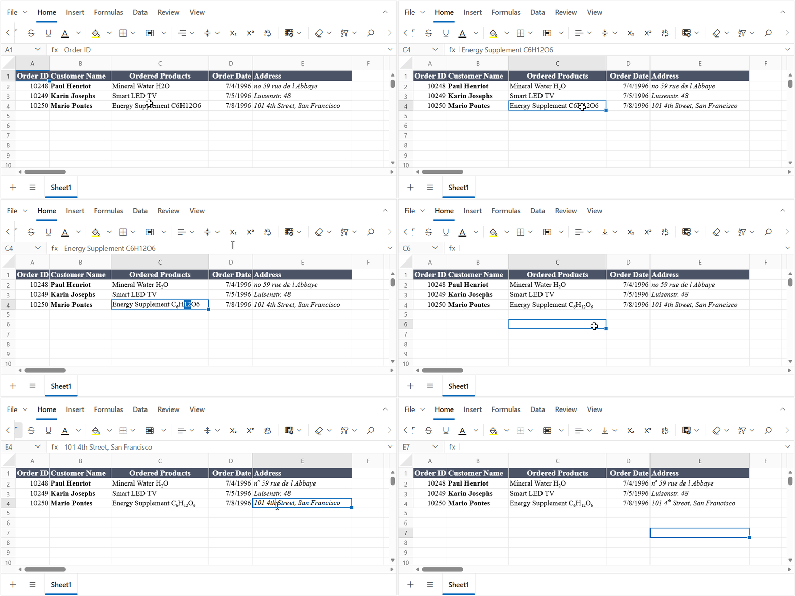
1. You can define the richText property directly while initializing the Spreadsheet. This is useful when you want the formatting to be applied when the data is loaded.

    cells: [
        {
            value: 'Annual Sales Report 2026 Highlights (Draft)',
            richText: [
                { text: 'Annual Sales Report ', style: { fontWeight: 'bold' } },
                { text: '2026', style: { color: '#0078D4' } },
                { text: ' Highlights', style: { textDecoration: 'underline' } },
                { text: ' (Draft)', style: { fontStyle: 'italic' } }
            ]
        }
    ]

1. You can also apply formatting dynamically using the updateCell method.

    spreadsheet.updateCell({
        richText: [
            { text: 'Premium Membership ', style: { fontWeight: 'bold', color: '#2E7D32' } },
            { text: 'valid until ', style: { fontStyle: 'italic' } },
            { text: '31', style: { textDecoration: 'underline' } },
            { text: 'st', style: { verticalAlign: 'super' } },
            { text: ' Dec 2026' }
        ]
    }, 'A5');

The following code example shows how to apply multiple rich text formats in cells of the Spreadsheet.

Composition API (~/src/App.vue)

<template>
  <ejs-spreadsheet ref="spreadsheet" :created="created" :showFormulaBar="false">
    <e-sheets>
      <e-sheet>
        <e-columns>
          <e-column :width="200"></e-column>
        </e-columns>

        <e-rows>
          <e-row>
              <e-cells>
                  <e-cell value="Plain Text"></e-cell>
              </e-cells>
          </e-row>

          <e-row>
              <e-cells>
                  <e-cell
                      value="Annual Sales Report 2026 (Draft)"
                      :richText="[
                          { text: 'Annual Sales Report ', style: { fontWeight: 'bold' } },
                          { text: '2026', style: { color: '#0078D4' } },
                          { text: ' (Draft)', style: { fontStyle: 'italic' } }
                      ]"
                  ></e-cell>
              </e-cells>
          </e-row>

          <e-row>
              <e-cells>
                  <e-cell
                      value="Customer Loyalty Program"
                      :richText="[
                          { text: 'Customer Loyalty ', style: { textDecoration: 'underline' } },
                          { text: 'Program', style: { fontFamily: 'Georgia', fontSize: '14pt' } }
                      ]"
                  ></e-cell>
              </e-cells>
          </e-row>

          <e-row>
              <e-cells>
                  <e-cell
                      value="Mineral Water H2O"
                      :richText="[
                          { text: 'Mineral Water H' },
                          { text: '2', style: { verticalAlign: 'sub' } },
                          { text: 'O' }
                      ]"
                  ></e-cell>
              </e-cells>
          </e-row>
      </e-rows>
      </e-sheet>
    </e-sheets>
  </ejs-spreadsheet>
</template>

<script setup>
import { ref } from "vue";
import { SpreadsheetComponent as EjsSpreadsheet, SheetsDirective as ESheets, SheetDirective as ESheet, RowsDirective as ERows, RowDirective as ERow, CellsDirective as ECells, CellDirective as ECell, ColumnsDirective as EColumns, ColumnDirective as EColumn } from "@syncfusion/ej2-vue-spreadsheet";

const spreadsheet = ref(null);

const created = () => {
    if (!spreadsheet.value) {
        return;
    }
    spreadsheet.value.updateCell(
        {
            value: 'Premium Membership valid until 31st Dec 2026',
            richText: [
                {
                    text: 'Premium Membership ',
                    style: {
                        fontWeight: 'bold',
                        color: '#2E7D32'
                    }
                },
                {
                    text: 'valid until ',
                    style: {
                        fontStyle: 'italic'
                    }
                },
                {
                    text: '31',
                    style: {
                        textDecoration: 'underline'
                    }
                },
                {
                    text: 'st',
                    style: {
                        verticalAlign: 'super'
                    }
                },
                {
                    text: ' Dec 2026'
                }
            ]
        },
        'A5'
    );
};
</script>

<style>
@import '../node_modules/@syncfusion/ej2-base/styles/tailwind3.css';
@import '../node_modules/@syncfusion/ej2-buttons/styles/tailwind3.css';
@import '../node_modules/@syncfusion/ej2-dropdowns/styles/tailwind3.css';
@import '../node_modules/@syncfusion/ej2-inputs/styles/tailwind3.css';
@import '../node_modules/@syncfusion/ej2-navigations/styles/tailwind3.css';
@import '../node_modules/@syncfusion/ej2-popups/styles/tailwind3.css';
@import '../node_modules/@syncfusion/ej2-splitbuttons/styles/tailwind3.css';
@import '../node_modules/@syncfusion/ej2-grids/styles/tailwind3.css';
@import "../node_modules/@syncfusion/ej2-vue-spreadsheet/styles/tailwind3.css";
</style>

Options API (~/src/App.vue)

<template>
  <ejs-spreadsheet ref="spreadsheet" :created="created" :showFormulaBar="false">
    <e-sheets>
      <e-sheet>
        <e-columns>
          <e-column :width="200"></e-column>
        </e-columns>

        <e-rows>
          <e-row>
              <e-cells>
                  <e-cell value="Plain Text"></e-cell>
              </e-cells>
          </e-row>

          <e-row>
              <e-cells>
                  <e-cell
                      value="Annual Sales Report 2026 (Draft)"
                      :richText="[
                          { text: 'Annual Sales Report ', style: { fontWeight: 'bold' } },
                          { text: '2026', style: { color: '#0078D4' } },
                          { text: ' (Draft)', style: { fontStyle: 'italic' } }
                      ]"
                  ></e-cell>
              </e-cells>
          </e-row>

          <e-row>
              <e-cells>
                  <e-cell
                      value="Customer Loyalty Program"
                      :richText="[
                          { text: 'Customer Loyalty ', style: { textDecoration: 'underline' } },
                          { text: 'Program', style: { fontFamily: 'Georgia', fontSize: '14pt' } }
                      ]"
                  ></e-cell>
              </e-cells>
          </e-row>

          <e-row>
              <e-cells>
                  <e-cell
                      value="Mineral Water H2O"
                      :richText="[
                          { text: 'Mineral Water H' },
                          { text: '2', style: { verticalAlign: 'sub' } },
                          { text: 'O' }
                      ]"
                  ></e-cell>
              </e-cells>
          </e-row>
      </e-rows>
      </e-sheet>
    </e-sheets>
  </ejs-spreadsheet>
</template>

<script>

import { SpreadsheetComponent, SheetsDirective, SheetDirective, ColumnsDirective, ColumnDirective, RowsDirective, RowDirective, CellsDirective, CellDirective } from "@syncfusion/ej2-vue-spreadsheet";

export default {
  name: "App",
  components: {
    "ejs-spreadsheet": SpreadsheetComponent,
    "e-sheets": SheetsDirective,
    "e-sheet": SheetDirective,
    "e-columns": ColumnsDirective,
    "e-column": ColumnDirective,
    "e-rows": RowsDirective,
    "e-row": RowDirective,
    "e-cells": CellsDirective,
    "e-cell": CellDirective
  },
  methods: {
    created: function () {
    const spreadsheet = this.$refs.spreadsheet;

    spreadsheet.updateCell(
          {
              value: 'Premium Membership valid until 31st Dec 2026',
              richText: [
                  {
                      text: 'Premium Membership ',
                      style: { fontWeight: 'bold', color: '#2E7D32' }
                  },
                  {
                      text: 'valid until ',
                      style: { fontStyle: 'italic' }
                  },
                  {
                      text: '31',
                      style: { textDecoration: 'underline' }
                  },
                  {
                      text: 'st',
                      style: { verticalAlign: 'super' }
                  },
                  {
                      text: ' Dec 2026'
                  }
              ]
          },
          'A5'
      );
    }
  }
};
</script>

<style>
@import "../node_modules/@syncfusion/ej2-vue-spreadsheet/styles/tailwind3.css";
@import "../node_modules/@syncfusion/ej2-base/styles/tailwind3.css";
@import "../node_modules/@syncfusion/ej2-buttons/styles/tailwind3.css";
@import "../node_modules/@syncfusion/ej2-dropdowns/styles/tailwind3.css";
@import "../node_modules/@syncfusion/ej2-inputs/styles/tailwind3.css";
@import "../node_modules/@syncfusion/ej2-navigations/styles/tailwind3.css";
@import "../node_modules/@syncfusion/ej2-popups/styles/tailwind3.css";
@import "../node_modules/@syncfusion/ej2-splitbuttons/styles/tailwind3.css";
@import "../node_modules/@syncfusion/ej2-grids/styles/tailwind3.css";
@import "../node_modules/@syncfusion/ej2-spreadsheet/styles/tailwind3.css";
</style>

Limitations

• Edit mode requirement: Formatting can be applied only while the cell is in edit mode. Selecting text outside of edit mode does not support subscript or superscript formatting.

Note

You can refer to our Vue Spreadsheet Editor feature tour page for its groundbreaking feature representations.

See Also

• Rows and columns
• Hyperlink
• Sorting
• Filtering
• Ribbon customization